In module 4 we predicted each speech sample from the last few, and found that what can't be predicted is the glottal kick. Rearranged, the predictor
equation reads \(x[n] = \sum_k a_k\,x[n-k] + e[n]\): a source \(e[n]\) going into something that rings. This page shows that this “something” is a filter made
entirely of poles, that each pair of poles is one formant, and that fitting it to a recording hands you the vocal tract's resonances,
good enough to take speech apart and rebuild it.
In module 4 the predictor analysed speech: given \(x[n]\), it produced the error \(e[n]\). Now read the same equation the other way, as a recipe for making a signal:
Each new output sample is the new input plus a weighted echo of what the filter itself just produced. The output is fed back into the input: this is feedback, and it
is why the model is called autoregressive (AR), “regressing on itself”.
Figure 1. The AR (all-pole) filter as a block diagram. Remove the feedback path and the output would just copy the input. With feedback, one input kick keeps echoing around the loop: the filter rings.
Feedback is how anything rings. A swing, the mass on a spring from module 3, a bell: their position now is set by their position a moment ago. A microphone held near its own loudspeaker howls
at one particular pitch for the same reason. With just two weights we already know exactly what the ring looks like. Module 4 showed that a decaying sinusoid \(\rho^n \sin(\omega n)\) obeys
\(x[n] = 2\rho\cos\omega\,x[n-1] - \rho^2 x[n-2]\). So two feedback weights make one resonance, ringing at frequency \(\omega\) and dying away at a rate set by \(\rho\):
$$a_1 = 2\rho\cos\omega, \qquad a_2 = -\rho^2, \qquad F = \frac{\omega}{2\pi}\,f_s, \qquad B \approx -\frac{f_s}{\pi}\ln\rho$$
\(F\) = resonance (formant) frequency in Hz, \(B\) = its bandwidth in Hz. The closer \(\rho\) is to 1, the longer the ring and the sharper the peak.
Impulse response: one kick in, the ring that comes out (first 20 ms)
Frequency response (0–8 kHz): one peak at \(F\), width \(B\)
Try pushing \(\rho\) towards 1: the ring lasts longer and the peak gets sharper and taller, exactly like light damping on the spring. Then push \(\rho\) past 1: each echo comes back
bigger than the last, and the output explodes. That is the howling microphone. A model of the vocal tract must keep \(\rho < 1\).
02 · Poles and the z-plane
Where formants live.
Engineers summarise a feedback filter with one piece of notation. Write \(z^{-1}\) for “delay by one sample”, so \(z^{-k}x[n]\) means \(x[n-k]\). The predictor equation, rearranged as
“input = output minus its echoes”, becomes a polynomial:
$$e[n] = x[n] - \sum_{k=1}^{p} a_k x[n-k] \quad\Longleftrightarrow\quad E(z) = A(z)\,X(z), \qquad A(z) = 1 - \sum_{k=1}^{p} a_k z^{-k}$$
$$H(z) = \frac{X(z)}{E(z)} = \frac{1}{A(z)}$$
\(A(z)\) is the prediction-error filter of module 4 (speech in, source out); \(H(z) = 1/A(z)\) is the vocal-tract filter (source in, speech out).
A polynomial can be factored into its roots. The roots of \(A(z)\) are the poles \(p_1, \dots, p_p\) of \(H(z)\): the values of \(z\) where the filter's response blows up.
Real filters have real weights, so complex poles always come in mirror-image pairs, \(p\) and \(p^*\). One such pair is exactly one resonance from section 01:
So we can draw a filter as dots on a plane, the z-plane. A pole's angle says which frequency it boosts (0 on the right, \(f_s/2\) = 8 kHz on the left).
Its distance from the centre says how sharply: near the unit circle means a narrow, tall formant; near the centre means a weak, broad one. Outside the circle, the filter is unstable.
Why the spectrum peaks near a pole: a geometric picture
The frequency response is the filter evaluated on the unit circle, \(z = e^{j\omega}\). Since \(H\) is one over a product, its size is one over a product of distances:
$$\bigl|H(e^{j\omega})\bigr| = \frac{1}{\prod_i \bigl|\,e^{j\omega} - p_i\,\bigr|} = \frac{1}{\text{product of the distances from the point } e^{j\omega} \text{ to every pole}}$$
Walk a point around the upper half of the unit circle from 0 Hz to 8 kHz. Whenever it passes close to a pole, one of the distances becomes tiny, the product drops, and \(|H|\) shoots up: a formant.
Try it: drag the poles, and use the frequency slider to walk the probe around the circle.
Drag a pole (\(\times\)). Its mirror image follows automatically.
Presets:
Frequency response \(|H|\) (0–5 kHz); dashed line = the probe's frequency
An AR filter is fully described by its poles. Each complex pole pair is one formant: angle → formant frequency, distance from the unit circle → bandwidth.
“All-pole” means the spectrum is shaped only by peaks, which is just what a vowel's spectrum looks like.
03 · Fitting real speech
The LPC envelope: from weights to formants.
Now put the pieces together. Take a 32 ms frame of real speech, find the best predictor weights exactly as in module 4 (autocorrelation method), and read them as \(A(z)\).
Then \(1/|A|\) draws a smooth curve over the spectrum (the LPC envelope), and the roots of \(A(z)\) give the formants. Nothing about formants was put in; they come out of
“predict the next sample as well as possible”.
$$\text{model power spectrum:}\quad \hat{S}(f) = \frac{G^2}{\bigl|A(e^{j2\pi f/f_s})\bigr|^2}$$
\(G^2\) = the leftover prediction-error energy, which sets the overall level.
Speech frame:
Poles of this fit
■ spectrum of the frame ■ LPC envelope (0–8 kHz)
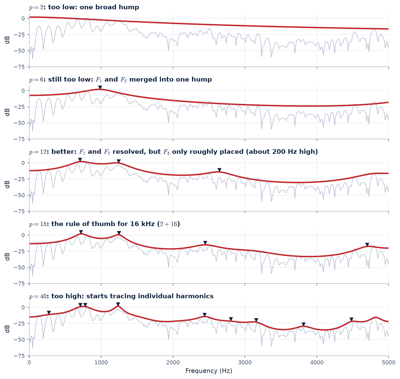
Figure 2. Choosing the order, on a 32 ms frame from the middle of /ɑ/ in “sharks” (CMU ARCTIC speaker ksp, Indian-English male, 16 kHz, pitch about 136 Hz here).
With too few poles there aren't enough to go round: at \(p = 6\), \(F_1\) and \(F_2\) merge into one hump near 990 Hz.
At \(p = 18\), the rule of thumb \(2 + f_s/1000\), the main formants each get their own pole pair (▼ at about 720, 1250 and 2450 Hz, plus a high resonance near 4700 Hz). With far too many poles the spare pairs start
latching onto individual harmonics, which belong to the source, not the filter. At \(p = 40\) the envelope sprouts a bump on the second harmonic (about 270 Hz) and splits \(F_1\) into two peaks (about 710 and 780 Hz) that hug neighbouring harmonics. Neither is a formant.
Why pre-emphasis? Toggle it in the demo. Without it, the voiced spectrum's steady downward tilt (about −6 dB/octave overall: roughly −12 from the glottal pulse, +6 from lip radiation) eats several
poles just to model the slope, and the high formants come out weak or missing. A gentle high-frequency boost first, \(x[n] - 0.97\,x[n-1]\), flattens the tilt so the poles are spent on formants.
04 · Take speech apart, put it back
Residual, resynthesis and an LPC vocoder.
Run the fit on every 10 ms frame of a whole sentence and we have a time-varying vocal-tract filter. Two things become possible:
Analysis: speech → \(A(z)\) → source
Pass the speech through the prediction-error filter \(A(z)\). The resonances are removed, leaving the residual: a buzz of glottal pulses (and noise where the speech is unvoiced).
Synthesis: source → \(1/A(z)\) → speech
Pass the residual back through the all-pole filter \(1/A(z)\). It puts the resonances back, and the speech comes out exactly as it went in.
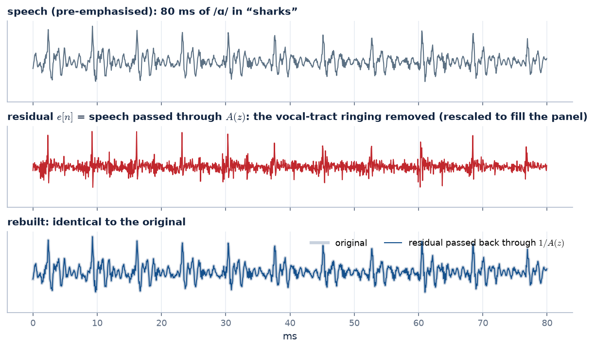
Figure 3. /ɑ/ in “sharks” with an 18-pole model updated every 10 ms. The residual is a train of sharp pulses, one per glottal closure (11 in these 80 ms, about 7.3 ms apart): the impulse-train source of module 3,
recovered from the recording alone. Passing it back through \(1/A(z)\) reproduces the speech exactly; over the whole sentence the difference is at the level of floating-point rounding (below −250 dB).
The exciting part comes next. If the residual is basically “pulses at the pitch, or noise”, we can throw it away and regenerate it from just three numbers per frame: voiced or not,
pitch, and loudness. Then we feed our home-made source through the 18 recorded filter weights. That is an LPC vocoder, the idea inside LPC-10 and the Speak & Spell. Because source and filter
are now separate, we can also change the source while keeping the filter:
Speech through \(A(z)\): the source. A buzzy, unintelligible-ish hum of glottal pulses, with hiss for /f/, /ʃ/ and /s/.
3 · Rebuilt
Residual through \(1/A(z)\). Indistinguishable from the original.
4 · LPC vocoder
Residual thrown away; replaced by clean pulses at the measured pitch (or noise), same filters. Robotic but clearly the same words and voice.
5 · Monotone
Pulses at a constant 100 Hz (this speaker talks at around 130–140 Hz): all intonation removed, the vowels and consonants untouched.
6 · Higher pitch
Pitch \(\times\,1.8\) with the same vocal tract: a higher voice, but not a “chipmunk”, because the formants haven't moved.
7 · Whisper
Noise everywhere, no pulses: the same filters turn it into whispered speech, as in the source–filter page's grid.
The vocoder sounds buzzy for two reasons: ideal pulses are a crude stand-in for the real glottal waveform, and a hard voiced/unvoiced switch can't do mixtures like /z/. That is precisely what
CELP fixed in 1985. It keeps the same all-pole filter, but instead of 3 numbers it sends a compact code for the residual itself, chosen so that the rebuilt speech sounds closest
to the original. Its descendants (VSELP, QCELP, and the ACELP family in GSM-EFR, AMR and its successors) have carried most mobile phone calls since the late 1990s.
05 · Limits
What an all-pole model can't do.
Anti-resonances (zeros). In nasals (/m/, /n/), the sound leaves through the nose while the closed-off mouth hangs off the side as a dead-end branch (in nasalised vowels it is the nasal cavity that branches off). A side branch absorbs energy at its own resonant frequencies, carving dips into the spectrum.
Dips need zeros (roots of a numerator polynomial), which an all-pole model doesn't have. It can only approximate a dip with extra poles. Pole–zero (ARMA) models handle this, at the cost of a much
harder fit. For most speech work the all-pole approximation, with a slightly higher order, is good enough.
High-pitched voices. With harmonics 250–400 Hz apart, the spectrum samples the envelope sparsely, and the poles get pulled towards individual harmonics, biasing the formant estimates.
A stationary frame. The model assumes the tract holds still for 20–30 ms. Fast transitions (stop releases, quick glides) are smeared.
The source is assumed flat. Real glottal pulses are smooth and lopsided, and some of their shape gets absorbed into \(A(z)\). Pre-emphasis helps; more careful
methods estimate the glottal pulse separately.
Looking ahead: back to the tubes
The concatenated-tube model of module 3 and the all-pole filter on this page are mathematically the same thing. The Levinson–Durbin recursion produces, along the way, a set of
reflection coefficients \(k_1, \dots, k_p\), one per joint in a chain of equal-length tubes. From those we can estimate the shape of the vocal tract from a recording alone.