On the source–filter page we saw that speech is a train of glottal kicks, each ringing through the vocal tract.
Ringing is predictable: once a bell has been struck, you know roughly what it will do next. This page turns that hunch into one of the most
successful ideas in speech technology, linear prediction: guess each new sample of a signal as a weighted sum of the last few.
We build it from scratch, starting with a game and a scatter plot, and end up with the method inside every mobile-phone call you've made.
Below are the last few samples of a signal. Click where you think the next sample will be (the dashed column). Then we reveal the true value, and also
the guess of a simple formula that only looks at the previous 12 samples. Play a few rounds of each signal.
Signal:
Click inside the dashed column to make your guess.
You will find the tone easy, the vowel fairly easy (it keeps going smoothly in the direction it was heading), and white noise impossible: the past
tells you nothing about the next value, and the best you can do is guess zero. The formula behaves exactly the same way. The rest of this page is about why,
and how that formula is built.
02 · Neighbours are related
A scatter plot of a signal against itself.
Here is a simple way to ask “does the past say anything about the future?”. Take every sample \(x[n]\) and pair it with the sample \(k\) steps later,
\(x[n+k]\). Plot all the pairs as dots. If the dots form a tilted line, knowing one sample tells you a lot about the other. If they form a
round blob, it tells you nothing. The tilt and tightness of the cloud are summarised by one number, the correlation:
$$r(k) = \frac{\sum_n x[n]\,x[n+k]}{\sum_n x[n]^2}$$
\(+1\): a perfect rising line · \(0\): a round blob · \(-1\): a perfect falling line
Pick a signal and slide the lag \(k\):
Signal:
correlation
\(r(k)\) for every lag (the dot marks the current \(k\))
Figure 1. The same idea for three signals (rows) at four lags (columns). 80 ms excerpts from CMU ARCTIC speaker ksp (an Indian-English male voice):
/ɑ/ from the exclamation “Ah”, /s/ from “see”.
White noise: round blobs at every lag, \(r \approx 0\). The past says nothing about the future.
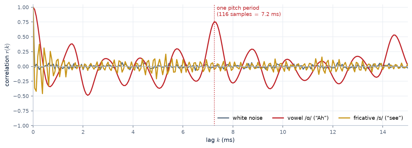
Vowel /ɑ/: at \(k = 1\) the dots hug a line (\(r = +0.96\)): consecutive samples are almost equal, because a 16 kHz sampler is much faster than the formant ringing.
By \(k = 11\) the line tilts the other way (\(r = -0.34\)): we've moved about half a cycle along the ringing of the first formant (\(F_1 \approx 660\) Hz, one cycle \(\approx 24\) samples).
At \(k = 116\), exactly one pitch period (7.25 ms, \(F_0 \approx 138\) Hz), the line comes back (\(r = +0.75\)): the waveform repeats.
Fricative /s/: weak, and negative at \(k = 1\) (\(r = -0.37\)). Its energy sits at high frequencies (most of it between about 4 and 7 kHz), so the waveform flips sign every couple of samples.
There's a bit of structure, but much less than for the vowel.
Figure 2. The correlation for every lag, from 0 to 15 ms. This curve is the autocorrelation. The vowel's curve oscillates at the formant frequencies and peaks again at the pitch period:
the two time scales of the source–filter model, visible in one plot.
For speech, neighbouring samples are strongly correlated, mainly because the vocal tract rings smoothly between glottal kicks. Correlation means the past
contains information about the present. That is the whole basis of prediction. White noise has no correlation, and nothing can predict it.
03 · From correlation to prediction
The best straight line through the scatter.
Go back to the lag-1 scatter of the vowel and tick show the best-fit line. That line is a predictor: read off \(x[n-1]\) on the horizontal axis and the line
gives a guess for \(x[n]\). The simplest possible predictor uses one weight:
$$\hat{x}[n] = a\,x[n-1], \qquad e[n] = x[n] - \hat{x}[n]$$
\(\hat{x}\) (“x-hat”) is the prediction; \(e[n]\) is the prediction error.
Which slope \(a\) is best? The one that makes the errors as small as possible overall, i.e. minimises the total squared error. Set its derivative to zero:
Now compare this with the definition \(r(k) = \sum_n x[n]\,x[n+k] \big/ \sum_n x[n]^2\), one piece at a time:
Numerator. Rename the time index, \(m = n-1\): \(\sum_n x[n]\,x[n-1] = \sum_m x[m]\,x[m+1]\). This is exactly the numerator of \(r(1)\): each sample times the one after it.
(Seen from the other sample it is the numerator of \(r(-1)\). That is fine: for a real signal \(r(-k) = r(k)\) always, because the same products are being summed. Only the
distance between the two samples matters, not which one comes first.)
Denominator. \(\sum_n x[n-1]^2\) is the energy of the signal shifted by one sample, and shifting doesn't change total energy. If the sums run over all \(n\)
(treating the frame as zero outside its window, the usual “autocorrelation method”), then \(\sum_n x[n-1]^2 = \sum_n x[n]^2\) exactly. If they only run over the samples inside a finite frame,
the two differ by one edge sample, a tiny difference in a frame of hundreds of samples.
$$a = r(1)$$
exactly, with the autocorrelation method; very nearly, if the sums stop at the frame edges (the “covariance method”).
So the best slope is just the correlation at lag 1. And how much does it help? Let's work out how much error energy is left.
Step 1: expand the square. Multiply out the error energy term by term:
Step 2: name the three sums. Write \(R(0) = \sum_n x[n]^2\) for the signal's energy. As we just saw, \(\sum_n x[n-1]^2\) is the same energy \(R(0)\), and
\(\sum_n x[n]\,x[n-1]\) is the lag-1 sum \(R(1) = r(1)\,R(0)\) (since \(r(1) = R(1)/R(0)\)). Substitute and take \(R(0)\) out as a common factor:
This is a parabola in \(a\) whose lowest point is at \(a = r(1)\): any other slope adds the extra \((a - r(1))^2\), which confirms the calculus without derivatives. Since \(r(1)^2\) can never exceed 1,
the error can never be negative, and it only reaches zero when \(|r(1)| = 1\), i.e. when the scatter is a perfect straight line.
Plugging in our three signals:
White noise
\(r(1) \approx 0 \Rightarrow a \approx 0\): the best guess is zero, and the error is as big as the signal. Gain 0 dB.
Fricative /s/
\(r(1) = -0.37\): guess the opposite sign, a lot smaller. Error energy \(1 - 0.13 = 87\%\). Gain \(\approx 0.6\) dB.
Vowel /ɑ/
\(r(1) = 0.96\): “next \(\approx\) previous”. Error energy \(1 - 0.92 = 8\%\). Gain \(\approx 11\) dB from one weight.
What is prediction gain?
The three cards above already used it. Prediction gain is the standard single number for how predictable a signal is. It compares the energy of the signal with the energy of what
the predictor leaves behind:
$$G_p = 10\log_{10}\frac{\sum_n x[n]^2}{\sum_n e[n]^2}\ \text{dB}, \qquad e[n] = x[n] - \hat{x}[n] = x[n] - \sum_{k=1}^{p} a_k\,x[n-k]$$
For one weight, section 03's algebra gives \(G_p = -10\log_{10}\bigl(1 - r(1)^2\bigr)\). For more weights it is computed from the actual error.
Reading the decibels: the gain says what fraction of the signal's energy was not predictable. (New to decibels, or wondering why audio uses them everywhere? See the extra page Why does audio live in decibels?)
prediction gain
error energy left
in words
0 dB
100 %
the past says nothing about the next sample
3 dB
50 %
half of it was predictable
10 dB
10 %
90 % was predictable
20 dB
1 %
99 % was predictable
30 dB
0.1 %
almost completely predictable
The values met on this page and the next ones, side by side:
signal
predictor
gain
why
white noise
any order
\(\approx 0\) dB
no correlation at any lag
fricative /s/
1 weight → 24 weights
0.6 → \(\approx 8\) dB
turbulent noise; only its spectral shape is predictable
vowel /ɑ/
1 weight → 18 weights
11 → \(\approx 24\) dB
two strong, low formants (\(F_1 \approx 660\), \(F_2 \approx 1200\) Hz): a smooth waveform
vowel /i/
1 weight → 18 weights
17 → \(\approx 27\) dB
a very low \(F_1\) (\(\approx 290\) Hz) makes it even smoother; its high \(F_2/F_3\) need the extra weights
averaged over a whole recording, vowels and consonants
pure tone
2 weights
\(\infty\) (in theory)
a sinusoid is exactly predictable (section 04)
A gain is only meaningful together with how it was measured. The same speech can give very different numbers depending on:
the order \(p\): more weights capture more resonances (try the slider in section 04), with diminishing returns beyond about \(2 + f_s/1000\);
the sampling rate: at a higher \(f_s\), neighbouring samples are closer together in time and more alike, so the gain rises;
pre-processing: pre-emphasis flattens the spectral tilt and removes the “easy” predictability, which explains 13 vs 24 dB for the same vowel;
the frame and how often the weights are refitted: speech changes, so the weights are re-estimated every 10–20 ms, and a reported gain is usually an average over frames;
what the predictor is allowed to see: a coder's decoder has only decoded (noisy) samples, so the gain it achieves in practice is lower than the ideal one computed on clean speech.
Prediction gain is the bridge from “speech is predictable” to “speech can be sent with fewer bits”. Every bit of quantiser resolution is worth about 6 dB, so a predictor with gain \(G_p\) lets a coder send the
error instead of the signal and save about \(G_p / 6\) bits per sample. That is the idea behind ADPCM on the codecs page.
04 · A weighted vote of the past
Why stop at one previous sample?
One weight can only express “the signal changes slowly”. A ringing resonance does more than that: it curves, overshoots and comes back. To follow a curve you need to know not just
where the signal is but where it was heading, which takes two previous samples. In fact, two weights predict a pure sinusoid perfectly, thanks to this identity:
Move \(\sin(\omega(n-2))\) to the right-hand side and we have the identity. \(\blacksquare\)
Three things to take from it:
It is a predictor with two weights. Writing \(x[n] = \sin(\omega n)\):
$$\hat{x}[n] = a_1\,x[n-1] + a_2\,x[n-2] \quad\text{with}\quad a_1 = 2\cos\omega,\;\; a_2 = -1$$
and the prediction is exact: zero error, for every \(n\). For our 200 Hz tone at 16 kHz, \(\omega = 2\pi \cdot 200/16000 = 0.0785\) rad, so \(a_1 = 2\cos(0.0785) = 1.994\) and \(a_2 = -1\).
This is what the demo below finds.
Amplitude and phase don't matter. The same proof works for \(x[n] = C\sin(\omega n + \varphi)\) (take \(A = \omega(n-1) + \varphi\) and multiply through by \(C\)). The weights depend only on the frequency.
So the two weights encode exactly one thing, which frequency is ringing. That is why they will later tell us where the formants are.
An intuition. Rearranged, the identity says \(x[n] + x[n-2] = 2\cos\omega \cdot x[n-1]\): the two neighbours of any sample add up to a fixed multiple of it. A slow oscillation
(\(\omega\) small, \(2\cos\omega \approx 2\)) means the neighbours almost average to the middle sample, i.e. the waveform is nearly straight locally. A fast oscillation bends sharply, so the neighbours fall well short of twice the middle value.
How many weights does speech need? The rule \(p \approx 2 + f_s/1000\)
This rule of thumb for the predictor order looks arbitrary, but every part of it has a meaning. It is a budget: count the resonances the predictor has to capture,
give each one two weights, and add a little extra for the overall slope of the spectrum.
Step 1 · One formant costs two weights
We just proved that a sinusoid is predicted exactly by two weights. A formant is a sinusoid that dies away, the decaying ring of a resonance. That also costs exactly two weights.
Multiply both sides of the identity by \(\rho^{\,n}\) (with \(0 < \rho < 1\) setting how fast the ring decays) and regroup the powers of \(\rho\):
$$\underbrace{\rho^{n}\sin(\omega n)}_{x[n]} = 2\rho\cos\omega\cdot\underbrace{\rho^{\,n-1}\sin\bigl(\omega(n-1)\bigr)}_{x[n-1]} \;-\; \rho^{2}\cdot\underbrace{\rho^{\,n-2}\sin\bigl(\omega(n-2)\bigr)}_{x[n-2]}$$
so a decaying ring is predicted exactly by \(a_1 = 2\rho\cos\omega\) and \(a_2 = -\rho^2\): one weight pair per resonance. \(\omega\) sets where the formant is, \(\rho\) how sharp it is.
Step 2 · How many formants are there to capture?
Recall the tube from the source–filter page: a 17.5 cm vocal tract has resonances at 500, 1500, 2500, 3500 Hz, …. They are spaced
about 1000 Hz apart, because the spacing is \(c/2L = 350/(2 \times 0.175) = 1000\) Hz. Real vowels push individual formants up and down, but the average density stays about one formant per kilohertz.
A signal sampled at \(f_s\) only contains frequencies up to \(f_s/2\) (the Nyquist frequency), so the predictor only has to deal with the formants below that:
$$\text{number of formants} \approx \frac{f_s/2}{1000\ \text{Hz}}$$
Why the extra 2? Besides its peaks, a voiced spectrum has an overall downward slope (about −6 dB per octave), from the smooth glottal pulse and the radiation at the lips
(section 05 of the source–filter page). A slope is not a resonance, but the predictor still has to model it, and a couple of extra weights take care of it.
(Pre-emphasis, which flattens that slope, is partly a way of saving those weights for the formants.)
The weight budget at 16 kHz: one box per formant below 8 kHz, two weights each, plus the tilt
\(8 \text{ formants} \times 2 \text{ weights} + 2 \text{ for tilt} = \mathbf{18}\). At 8 kHz sampling only \(F_1\)–\(F_4\) lie below the 4 kHz Nyquist limit, giving \(4 \times 2 + 2 = \mathbf{10}\).
Sampling rate \(f_s\)
Nyquist \(f_s/2\)
Formants below it
Order \(p\)
Typical use
8 kHz
4 kHz
\(\approx 4\)
10
telephone speech, LPC-10, most phone codecs
10 kHz
5 kHz
\(\approx 5\)
12
classic speech-analysis setups
16 kHz
8 kHz
\(\approx 8\)
18
wideband speech, most speech corpora (e.g. CMU ARCTIC), ASR
It's a guideline, not a law. The 1000 in the formula is really the formant spacing \(c/2L\), so it depends on the speaker. A shorter (female or child) tract has formants about
1200–1500 Hz apart, so slightly fewer of them fit below Nyquist and a slightly lower order suffices. The high formants are also weak, so in the demo below the gain for /ɑ/ is already
within about 2 dB of its maximum by \(p \approx 12\). Too low an order merges or misses formants. Too high an order starts fitting individual harmonics and noise, giving
spurious peaks. The rule puts you safely in between.
Putting it together, the general predictor is a weighted vote of the last \(p\) samples:
It is called linear prediction because the guess is a weighted sum: no squares, no thresholds, nothing fancy. Try different orders:
Signal:
■ actual ■ predicted ■ error (same scale), first 25 ms
Prediction gain vs. order (dot = current \(p\))
The weights \(a_1, \dots, a_p\)
prediction gain
error energy left
What to notice:
Tone: \(p = 2\) is perfect, and the gain shoots off the chart (limited only by the rounding of the stored samples). Extra weights add nothing to the gain,
but notice that they are not zero (see the box below).
Vowels: the gain climbs quickly, about 2 weights per formant, then levels off around \(p \approx 12\)–18. Beyond that the leftover error is the part that is genuinely new each period: the glottal kicks.
Fricative: about 8 dB at most. Turbulent noise is mostly unpredictable, but its spectral shape (where the noise energy sits) is still captured by the weights.
Noise: zero gain at every order. No pattern, nothing to exploit.
Why aren't the extra weights zero for the tone when \(p > 2\)?
Because there is no longer one best answer: there are infinitely many, all perfect. For a sinusoid, any three consecutive samples are tied together by the identity itself
(written one step earlier):
So we can add any multiple \(\lambda\) of that zero to the two-weight predictor without changing a single prediction. With \(c = \cos\omega\), every member of this family is exact:
For our 200 Hz tone: \(\lambda = 0\) gives \((1.994, -1, 0)\); \(\lambda = -2c\) gives \((0,\, 2.975,\, -1.994)\), a predictor that ignores the most recent sample entirely; and the demo shows
\((1.552,\, -0.120,\, -0.441)\), which is \(\lambda \approx -0.44\). All three have zero error.
In matrix terms, the normal-equation matrix for a pure tone has rank 2. For \(p = 3\) it is singular (one eigenvalue is exactly zero), so the equations don't pin down a unique solution.
The solver needs a tie-breaker. A tiny amount of “prefer small weights” (regularisation) would select the family member with the smallest total
\(\sum_k a_k^2\), which is \(\lambda = -2c/(1 + 2c^2) \approx -0.667\), i.e. \((1.327,\, 0.330,\, -0.667)\). That spreads the weight over all the lags rather than zeroing the extra ones.
The demo lands on a different member for a mundane reason: its samples are stored rounded to 4 decimals, and that rounding acts like a tiny, periodic “noise” that makes the matrix very slightly
non-singular, so the rounding, not the regulariser, breaks the tie. Either way, the extra weights are not zero.
Real signals don't have this problem. Speech, noise, even a tone with a little added noise, carry information in more than two dimensions, so the matrix is invertible and the
weights are unique. The pure tone is the special case that shows exactly how much structure a signal has: two numbers' worth, so a third weight is redundant.
05 · Finding the weights
Least squares, with the same trick as before.
With one weight we set a derivative to zero and got \(a = r(1)\). With \(p\) weights we do exactly the same thing, once for each weight: minimise the total squared error
Each condition says “the error must be uncorrelated with \(x[n-i]\)”: whatever is left over shouldn't still be predictable from the past. Written out, they are \(p\) linear equations that only involve the correlations \(r(k)\) we already know how to compute:
$$\sum_{k=1}^{p} a_k\, r(|i-k|) = r(i), \qquad i = 1,\dots,p$$
the normal equations, a.k.a. the Yule–Walker equations. For \(p = 2\):
$$\begin{bmatrix} r(0) & r(1) \\ r(1) & r(0) \end{bmatrix}\begin{bmatrix} a_1 \\ a_2 \end{bmatrix} = \begin{bmatrix} r(1) \\ r(2) \end{bmatrix}$$
The absolute value in \(r(|i-k|)\) is the symmetry from section 03 again: \(r(-k) = r(k)\), so only the distance between the two samples counts. The matrix therefore has the same value along every diagonal (a Toeplitz matrix), and it is also symmetric. That structure lets the
Levinson–Durbin recursion solve the system in about \(p^2\) operations instead of \(p^3\): fast enough for 1970s chips to do it 50 times a second.
(The demos on this page solve the same least-squares problem directly, in your browser, each time you move a slider.)
In practice (the “autocorrelation method”): take a 20–30 ms frame, apply a smooth window (Hamming) and usually a little pre-emphasis (to flatten the spectral tilt),
compute \(r(0), \dots, r(p)\), solve for the weights, move on 10 ms, repeat. Speech changes, so the weights are re-estimated for every frame.
06 · History
From a lost planet to your phone.
Did prediction start in astronomy? Mostly yes. The fitting machinery (least squares, which is exactly how we found the weights) was born predicting the motion
of a celestial body. The specific idea of predicting a signal from its own past came in the 1920s, again from a sky-watching problem (sunspots), and reached speech in the 1960s.
1801–1809
Gauss and the lost planet Ceres. Ceres was spotted in January 1801, then lost in the Sun's glare after only 41 days of observations. The 24-year-old Carl Friedrich Gauss fitted an orbit to those few noisy positions by least squares and predicted where it would reappear; it was found there on 31 December 1801. Legendre published least squares first (1805); Gauss published his method in 1809.
1927
Yule and the sunspots. Udny Yule modelled the yearly sunspot numbers as each value predicted from the previous two plus a random disturbance. This was the first autoregressive (AR) model, and the same structure as our predictor.
1931
Walker generalised it to more past values while studying atmospheric pressure at Darwin, giving the Yule–Walker equations, the very equations of section 05.
1941–1949
Kolmogorov and Wiener founded the theory of optimal prediction of random signals. Wiener's version came from a wartime problem: predicting where an aircraft would be by the time an anti-aircraft shell arrived.
1947
Levinson found the fast recursion for the Toeplitz equations (refined by Durbin in 1960).
1966–1971
Speech arrives. Fumitada Itakura and Shuzo Saito at NTT in Japan, and Bishnu Atal and Manfred Schroeder at Bell Labs, independently realised that the vocal tract makes speech highly predictable, so a predictor's weights are a compact description of the filter. Atal & Hanauer's 1971 paper “Speech analysis and synthesis by linear prediction of the speech wave” became the field's foundation.
1975
John Makhoul's tutorial “Linear prediction: a tutorial review” makes LPC the standard tool of speech processing.
1978
Texas Instruments' Speak & Spell toy talks using a single LPC synthesis chip: the source–filter model, in a children's toy.
1984
LPC-10 (US standard FS-1015) sends intelligible speech at 2.4 kbit/s: per frame just ~10 predictor weights, a pitch, a voicing flag and a gain.
1985 →
CELP (Schroeder & Atal) adds a smarter way to code the prediction error. Its descendants (GSM's enhanced full-rate codec, AMR, EVS, …) and close linear-predictive relatives such as the speech mode of Opus run in essentially every mobile phone today.
First: what are sunspots, and why did anyone care?
Sunspots are dark patches on the Sun's visible surface (the photosphere). They are dark only by comparison: at roughly 3,500–4,500 K they are cooler than the
surrounding surface at about 5,800 K, and on their own they would glow bright orange. They form where bundles of intense magnetic field push up through the surface and choke the
churning convection that normally carries heat up from below. Big ones are several times wider than the Earth. They last from days to weeks, appear in groups, usually in two
bands either side of the solar equator, and are carried across the disk by the Sun's rotation (about 27 days as seen from Earth).
Figure 3. What is being counted. A sunspot has a dark core (the umbra) and a lighter, striped rim (the penumbra), and a large one can swallow several Earths.
Rudolf Wolf's count weights each group ten times more than an individual spot, because small spots come and go and are easy to miss, while groups are a steadier sign of activity.
\(R\) is computed each day from what is visible that day.
What does a “yearly sunspot number” mean?
It is not a count of how many different spots appeared during the year. It is the average of the daily numbers:
$$R_{\text{day}} = k\,(10\,g + s) \quad\text{(from the visible half of the Sun on that day)}, \qquad R_{\text{year}} = \frac{1}{\text{days}}\sum_{\text{days in the year}} R_{\text{day}}$$
Nobody tracks individual spots from day to day. A long-lived group is simply counted again on every day it is visible: about two weeks as the Sun's rotation carries it across the disk, and again
if it survives to come back round about 27 days later. So the yearly number measures how spotted the Sun looks on a typical day of that year, a level of activity.
For example, 1957's record yearly value of about 190 corresponds to an average day showing something like 12 groups and 70 spots (\(10 \times 12 + 70 = 190\)). The factor \(k\) puts different observers
and telescopes on a common scale. Today a worldwide network of stations contributes, which also covers days when one site is clouded out.
Counting them: 250 years of patient observation
Sunspots were noted with the naked eye in Chinese chronicles over two thousand years ago, and drawn through the first telescopes by Harriot, Galileo, Scheiner and Fabricius in 1610–1611.
The cycle was discovered almost by accident: Heinrich Schwabe, an apothecary and amateur astronomer, counted spots on every clear day from 1826, hoping to catch an unknown
planet crossing the Sun. He found no planet, but in 1843 he announced that the number of spots rises and falls over about ten years. In 1848 Rudolf Wolf in Bern (later Zürich) defined
the sunspot number above, began a systematic daily record, and painstakingly reconstructed earlier years from old observations: monthly back to 1749, yearly back to 1700. His successor
Alfred Wolfer continued it, which is why Yule speaks of “Wolfer's sunspot numbers”. The series is still maintained today (by the Royal Observatory of Belgium) and is one of the longest
scientific records that exists.
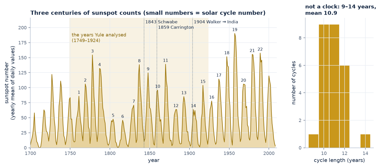
Figure 4. The yearly sunspot record, 1700–2008, with the solar cycles numbered from 1 (starting 1755). The shaded band is the stretch Yule analysed. Right: how long each cycle lasted,
measured minimum to minimum. They range from 9 to 14 years, mean 10.9. The peaks vary even more, from about 45 to 190. A regular cycle that refuses to keep regular time: that is exactly
the puzzle described below.
Why did predicting sunspots matter then?
🧭 Compasses and telegraphs
In 1852 Edward Sabine (and independently Wolf and Gautier) showed that disturbances of the Earth's magnetic field, the restless twitching of compass needles, rise and fall in step with the
sunspot cycle. Then in September 1859 Richard Carrington saw a brilliant flare on the Sun, and within a day the largest magnetic storm on record struck. Aurorae were seen near the tropics,
and telegraph systems across Europe and America failed, threw sparks, or kept working on currents induced by the storm alone. The Sun clearly mattered for the new electrical technologies.
🌾 Weather, harvests and prices
If the Sun's output varied with the cycle, perhaps the weather did too. William Herschel suggested in 1801 that English wheat prices were higher in years with few sunspots. In the 1870s the economist
W. S. Jevons argued that trade crises recurred with the sunspot cycle (the “sunspot theory” of business cycles). Most such links did not survive careful testing, but for decades
the sunspot cycle was a prime suspect for anything that seemed to repeat.
🌧️ The Indian monsoon
When the monsoon failed, millions died: in the famines of 1876–78 and 1899–1900. Forecasting the monsoon became a priority of the India Meteorological Department (H. F. Blanford issued
long-range forecasts from 1886), and sunspots were among the predictors examined. In 1904 Gilbert Walker, a Cambridge mathematician, became Director-General of Observatories in India
with exactly this task. Searching worldwide weather records for anything that foretold the monsoon, he discovered the Southern Oscillation, a see-saw of air pressure across the Pacific
(Darwin vs. Tahiti), today known as part of ENSO (El Niño) and still a key monsoon predictor. His 1931 paper was built to analyse exactly such series.
📈 Statistics itself
With over two centuries of numbers and an obvious but irregular rhythm, the sunspot series became the standard test case for methods of finding cycles in data. Yule was worried about
how easily one finds spurious patterns in time series (his 1926 paper asked “Why do we sometimes get nonsense-correlations between time-series?”). The sunspots were
the natural place to show that a better model was needed.
The question has never gone away. Solar storms now threaten satellites, GPS, radio links and power grids: the March 1989 storm blacked out the Québec grid for nine hours. Space-weather centres
forecast the sunspot cycle (cycle 25 reached its maximum around 2024–25), and autoregressive models in Yule's spirit are still among the tools used.
How Yule and Walker actually did it
The equations in sections 03–05 were not invented for speech. They were worked out by two statisticians trying to understand sunspots, and seeing how they did it makes the
method feel much less arbitrary. We can redo their analysis on the same data (the yearly sunspot numbers of 1749–1924 that Yule used).
The puzzle: is the 11-year sunspot cycle a hidden sine wave?
Astronomers had long known that sunspots come and go in a cycle of roughly 11 years. Around 1900 the standard tool for finding such cycles was Arthur Schuster's periodogram
(essentially a Fourier transform). It assumed the data were one or more perfect sine waves plus independent measurement errors. But the sunspot cycle doesn't behave like that.
Its length wanders between about 9 and 14 years and its peaks vary wildly in height. A perfect sine wave can't drift like that: the “errors” in one year have no effect on the next.
Yule's idea (1927): a pendulum pelted with peas
George Udny Yule proposed a different picture, in a famous image. Imagine a pendulum swinging in a room, and some boys who keep pelting it with peas. Each pea doesn't add an error on top of
the swing. It knocks the pendulum, and the pendulum carries that knock forward into all its future swinging. The motion still looks roughly periodic (a pendulum has a natural period), but
its timing and size wander irregularly, just like sunspots.
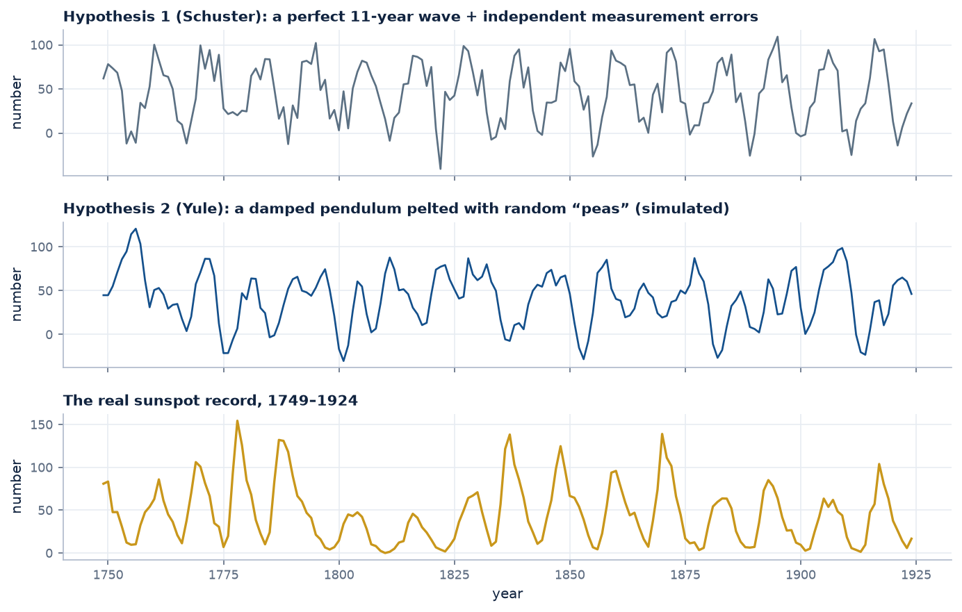
Figure 5. The two hypotheses, simulated, next to the real data. Schuster: the cycle is perfectly regular, and the noise only jiggles each point. Yule: random knocks fed through a
damped two-step “pendulum” (the model he fitted, below) produce cycles whose length and height wander, much more like the real record. (The simulated series can dip below zero
because the models are linear; real counts can't.)
Try it yourself: throw some peas.
Set the peas to zero and the pendulum just swings down to rest: without disturbances the cycle dies away. The random knocks are what keep it going and what make it irregular.
How Yule fitted it: correlation and least squares
A damped pendulum, written one time step at a time, says that this year's value is a fixed mix of the last two years' values. So Yule wrote, with \(x_t\) the sunspot number in year \(t\)
(measured from its average) and \(\varepsilon_t\) the year's random “pea”:
$$x_t = a_1\,x_{t-1} + a_2\,x_{t-2} + \varepsilon_t$$
This is exactly our two-weight predictor from section 04, with years instead of samples and peas instead of glottal kicks.
To find \(a_1\) and \(a_2\) he did what we did. First he checked that neighbouring years are correlated, with the same kind of lagged scatter plot as in section 02:
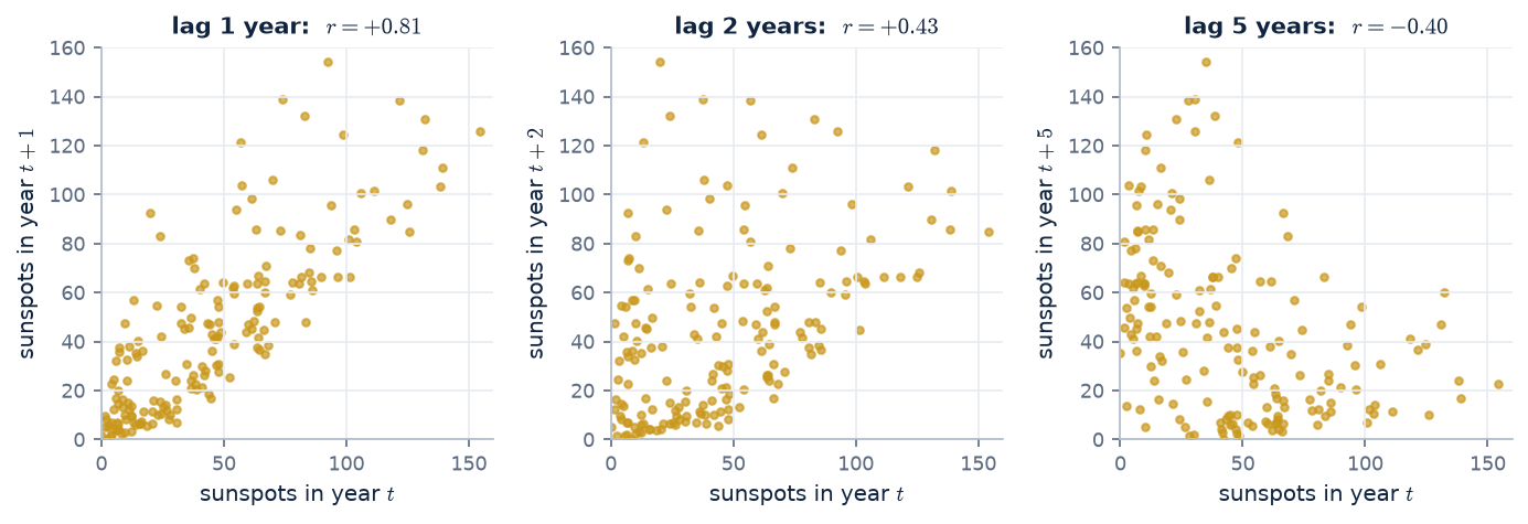
Figure 6. Sunspot number in year \(t\) against year \(t+k\). One year apart they are strongly related (\(r = +0.81\)). Two years apart, less so (\(+0.43\)). Five years apart,
half a cycle, they are anti-correlated (\(-0.40\)), just like the vowel at half a formant period in Figure 1.
Then he chose the weights that minimise the squared prediction error (least squares, Gauss's tool from the Ceres story), exactly as in section 05. On his data this gives:
$$x_t = 1.34\,x_{t-1} - 0.65\,x_{t-2} + \varepsilon_t$$
Our recomputation on the same years gives 1.336 and −0.650. Yule (1927) reported coefficients of about 1.34 and −0.65.
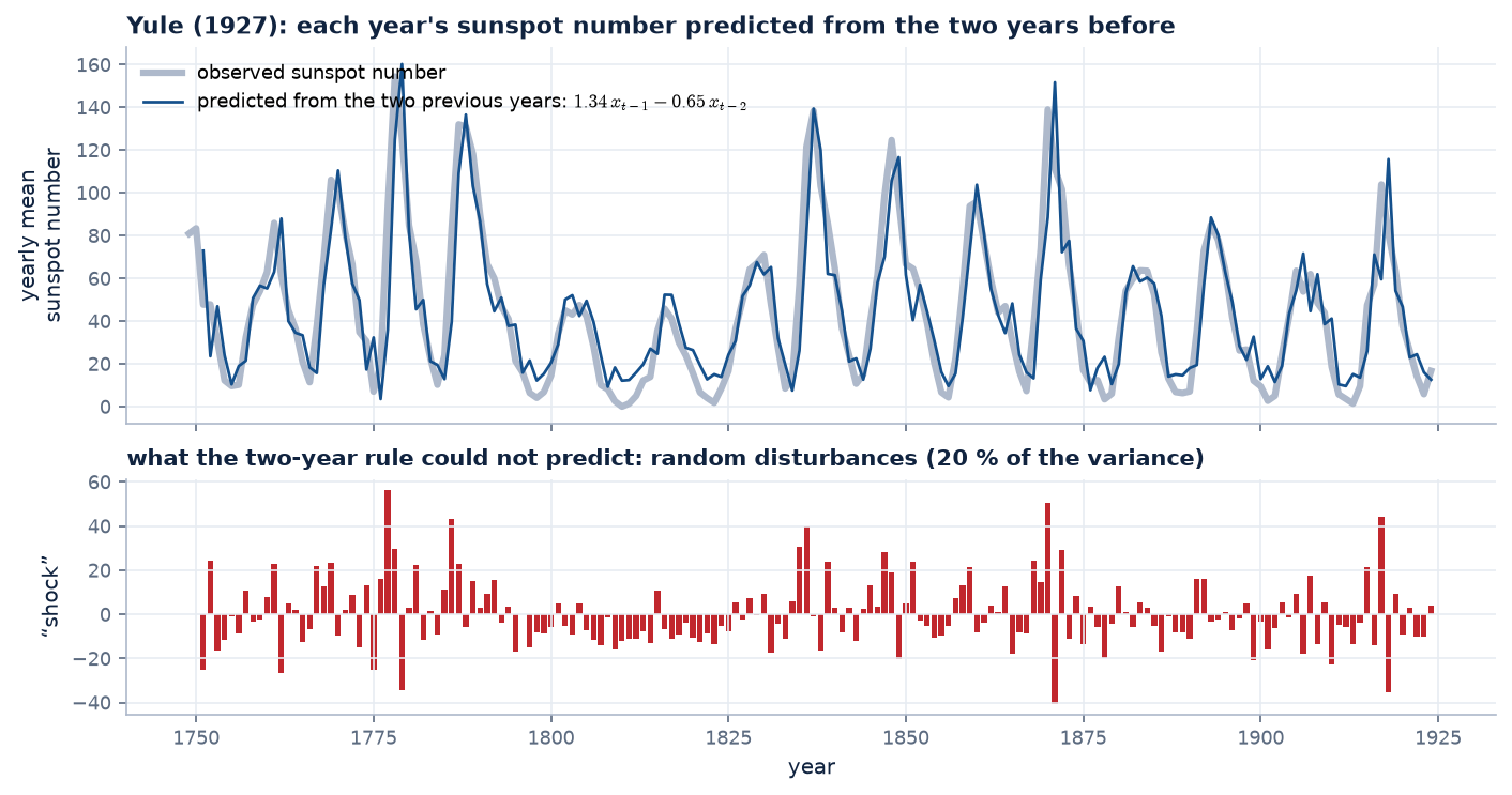
Figure 7. Yule's predictor in action: each year predicted from the two before. The prediction tracks the cycle closely. What it can't predict (red) is the random “peas”:
about 20 % of the variance, versus 35 % if only one previous year is used.
And the two numbers have a physical meaning, the same one they have for speech. Using section 04's result for a decaying ring, \(a_1 = 2\rho\cos\omega\) and \(a_2 = -\rho^2\):
$$\rho = \sqrt{0.650} = 0.81, \qquad \cos\omega = \frac{1.336}{2 \times 0.81} \;\Rightarrow\; \omega = 0.594 \text{ rad/year} \;\Rightarrow\; \text{period} = \frac{2\pi}{\omega} = 10.6 \text{ years}$$
The fitted “pendulum” has a natural period of 10.6 years, the sunspot cycle, and loses about 19 % of its swing each year (\(\rho = 0.81\)).
In speech terms, Yule found the sunspot record's single formant: its resonant frequency and its damping, read directly off two prediction weights. This is the same calculation that gives \(F_1\) from a vowel, some 40 years before anyone did it for speech.
Walker's step (1931): let the correlations do the work
Sir Gilbert Walker, studying the Southern Oscillation (the see-saw of air pressure across the Pacific, measured at Darwin), extended Yule's model to any number of past values and noticed something elegant.
Take the model, multiply both sides by an earlier value \(x_{t-j}\), and average over all \(t\):
$$x_t\,x_{t-j} = \sum_{k=1}^{p} a_k\, x_{t-k}\,x_{t-j} + \varepsilon_t\,x_{t-j} \quad\xrightarrow{\text{average}}\quad r(j) = \sum_{k=1}^{p} a_k\, r(j-k) + 0$$
The pea term averages to zero because this year's pea can't be correlated with a value from an earlier year: it hadn't been thrown yet.
Two consequences:
The weights come straight from the correlations. Writing that equation for \(j = 1, \dots, p\) gives \(p\) equations in the \(p\) unknown weights, which are exactly the normal equations of section 05.
Hence the name Yule–Walker equations. For \(p = 2\):
$$\begin{bmatrix} 1 & r(1) \\ r(1) & 1 \end{bmatrix}\begin{bmatrix} a_1 \\ a_2 \end{bmatrix} = \begin{bmatrix} r(1) \\ r(2) \end{bmatrix} \quad\Rightarrow\quad \begin{bmatrix} a_1 \\ a_2 \end{bmatrix} = \begin{bmatrix} 1.33 \\ -0.64 \end{bmatrix}$$
using the sunspot correlations \(r(1) = 0.81\), \(r(2) = 0.43\).
The correlations obey the same recursion as the data. For \(j > p\) the same equation says \(r(j)\) is built from earlier correlations with the same weights. So the
correlogram of a pelted pendulum is itself a damped oscillation at the pendulum's period. That gave a direct test of the model:
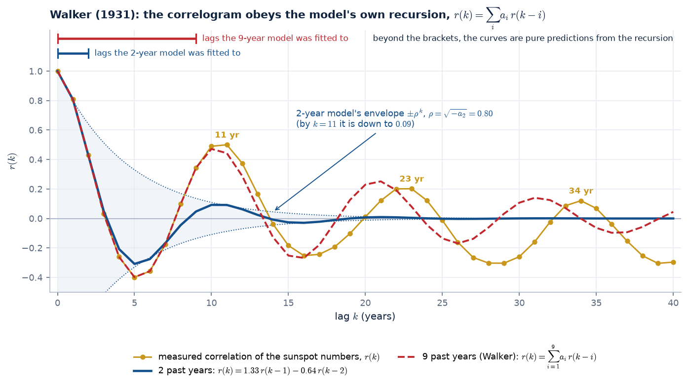
Figure 8. Walker's test on the sunspot record. Each model is fitted only to the lags under its bracket; everything to the right is predicted by running the recursion forward.
The measured correlogram (gold) peaks at 11, 23 and 34 years: the solar cycle shows up as a slow ring in the correlations. The two-year model (blue) matches the lags it was fitted to, but its
pole radius \(\rho = \sqrt{-a_2} = 0.80\) makes it lose 20 % of its amplitude every year (dotted envelope \(\pm\rho^k\)), so by the first peak it has almost died: the real cycle is more regular than a two-weight pendulum.
With nine past years (red, Walker's generalisation) the predicted correlogram keeps ringing with the data for decades, slowly drifting out of phase. More weights capture more structure,
the same lesson as the order slider in section 04.
correlations → Yule–Walker (normal) equations → least squares: identical
what the weights reveal
one resonance: period 10.6 years
several resonances: the formants
typical order
2 (Yule), more (Walker)
10–18
When Itakura, Saito and Atal applied this to speech in the late 1960s, the pendulum had become a vocal tract and the peas had become glottal pulses, but the mathematics was Yule's and Walker's, unchanged.
07 · What can't be predicted
The leftover is the source.
Here is linear prediction run on real speech. Look at what is left after the predictor has done its best:
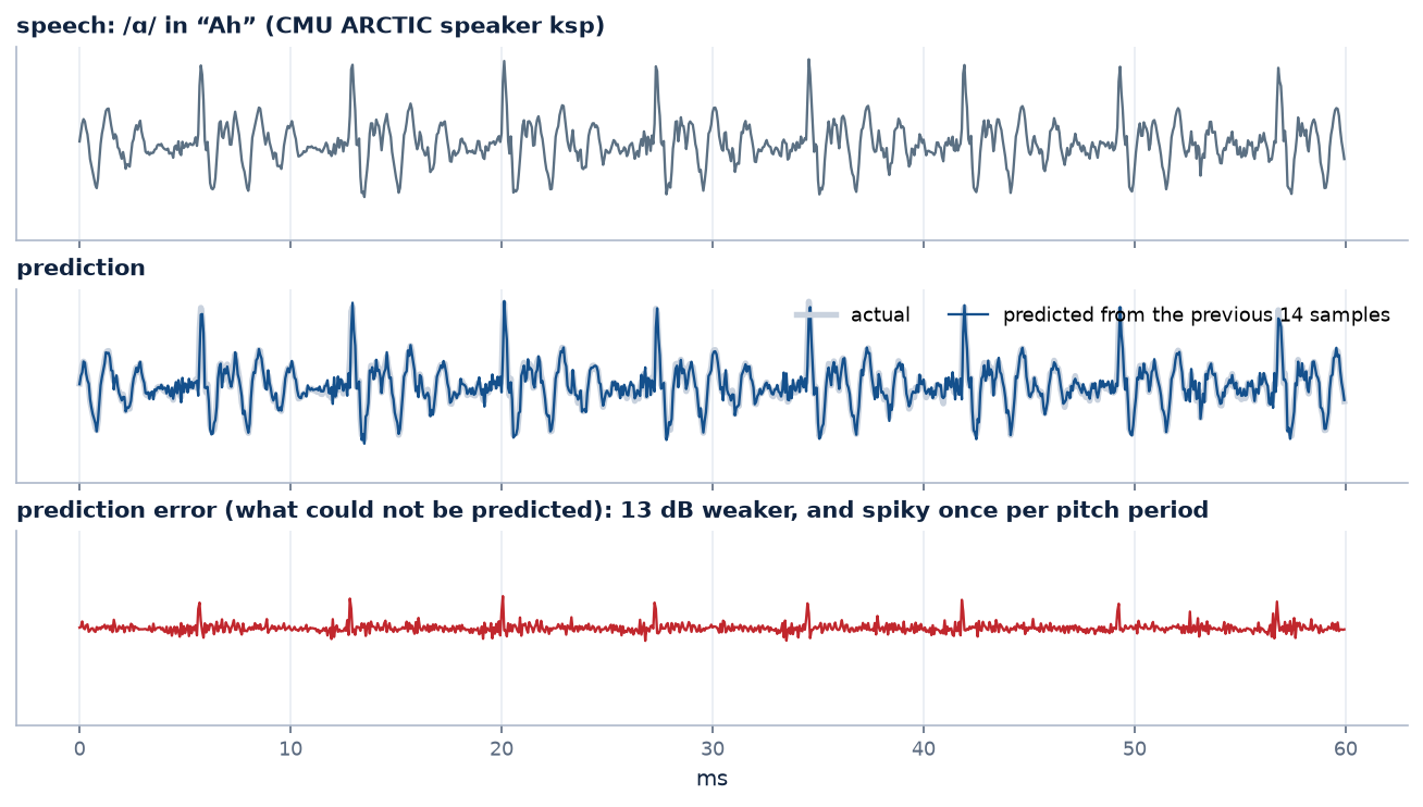
Figure 9. 60 ms of /ɑ/ in the exclamation “Ah” (CMU ARCTIC speaker ksp, lightly pre-emphasised), predicted from the previous 14 samples. The prediction (blue) follows the speech closely. The error (red, same scale)
is about 13 dB weaker and almost flat, except for a burst once every pitch period (every 7.25 ms here). (The gain here, 13 dB, is lower than the ~24 dB in the demo above because the speech was pre-emphasised first. That removes the easy, slowly varying part, leaving the predictor the harder job of modelling the resonances, which is what we want for analysis.)
Remember the source–filter picture: each period, a glottal kick starts a ringing. The ringing follows smoothly from what came before, so the predictor
learns it and removes it. The kick arrives out of nowhere, so it can't be predicted, and it stays in the error. Prediction splits speech back into its two parts:
What was predictable → the filter
The weights \(a_1,\dots,a_p\) describe the vocal tract's ringing: its resonances, its formants.
What wasn't → the source
The error \(e[n]\) is close to the impulse train of glottal kicks (or the noise, for /s/).
Rearranging the definition of the error gives the model that ties it all together:
Read that equation as a filter driven by \(e[n]\) and it is the source–filter model: an autoregressive (all-pole) filter. Next we'll see how its weights become
poles, each pair of poles one formant; how its frequency response draws the smooth envelope over a real spectrum; and how to pick the order. Then we close the loop with the tubes:
the same weights can be turned into the reflection coefficients of a concatenated-tube vocal tract.
Check your understanding
1. Why is \(r(1)\) so close to 1 for a vowel sampled at 16 kHz, and what would happen at 48 kHz?
Between two samples only \(1/16000\) s passes, while the dominant ringing (\(F_1 \approx 700\) Hz) takes over 1 ms per cycle, so consecutive samples barely change. At 48 kHz they would be even closer, so \(r(1)\) even nearer 1. High sampling rates make speech more predictable sample-to-sample.
2. The best one-weight predictor for /s/ had a negative weight. What does that mean physically?
Its energy is concentrated at high frequencies, around a quarter of the sampling rate or more, so the waveform tends to flip sign from one sample to the next. “Guess the opposite of the last sample” is the best one-step strategy.
3. Why does adding more weights beyond \(p \approx 18\) barely improve the prediction of a vowel?
The predictable part (the ringing of a few resonances) is already captured. What remains is mostly the glottal kicks, which are new information each period. A predictor reaching back over a whole pitch period (~100–150 samples for a male voice at 16 kHz; 116 for our /ɑ/) could exploit that too: this is the long-term (pitch) predictor used in CELP codecs.
4. Would linear prediction help compress music? A recording of rain?
Music: yes, tonal music is highly predictable (lossless codecs such as FLAC use linear prediction). Rain: hardly. It is noise-like, so like white noise or /s/ the gain would be small; only its spectral shape could be captured.