Every phone call, voice message and video meeting sends your voice as a stream of bits, and every bit costs radio spectrum, network capacity, battery and money.
Speech coding is the art of sending as few bits as possible while the person at the other end still hears you. This page starts from the most obvious
ways to save bits, shows where they break down, and then uses the LPC model of modules 4–5 to go down from 256 kbit/s to under 3 kbit/s. Every step
comes with audio you can listen to.
Follow your voice on a phone call. It is turned into numbers, squeezed, sent, unsqueezed and turned back into sound:
Figure 1. The speech communication chain. The ADC turns the voice into numbers. The encoder squeezes them into as few bits as it can, the channel carries the bits,
and the decoder rebuilds a signal from them. The decoder only ever sees the bits, so whatever the encoder throws away is gone for good.
What is a bit rate?
A digital audio signal is a sequence of numbers: samples, taken \(f_s\) times per second, each stored with \(b\) bits. The bits per second needed to send it raw is simply
$$\text{bit rate} = f_s \times b \times \text{channels}$$
this page's speech sample, resampled to 16 kHz: \(16\,000 \times 16 \times 1 = 256\,000\) bits/s = 256 kbit/s. (The raw recording, at 48 kHz and 32 bits, was \(1536\) kbit/s.) A music CD: \(44\,100 \times 16 \times 2 = 1411\) kbit/s.
📶 Radio spectrum is finite
A cell tower has a fixed slice of spectrum to share among everyone nearby. Halve the bits per call and roughly twice as many people can talk at once.
🔋 Bits cost energy
Transmitting is one of the most power-hungry things a phone does. Fewer bits means less time with the radio on, and longer battery life.
🌐 Weak links and storage
A low bit rate still gets through on a poor connection, a satellite link or a crowded network. An hour of raw 16 kHz speech is 115 MB; at 8 kbit/s it is 3.6 MB.
The catch: the listener must still understand the words, recognise the speaker, and not be annoyed. Engineers use rough quality classes: toll quality (as good as a traditional phone line),
communication quality (clearly intelligible, noticeably degraded) and synthetic quality (intelligible, but robotic). The rest of this page is a race down
the bit rate while trying to stay in the best class possible.
02 · The two obvious knobs
Fewer bits per sample, or fewer samples per second.
The formula has two knobs that don't need any knowledge of speech at all. Both work on the waveform directly: they try to reproduce the exact shape of the signal, sample by sample.
Knob 1: fewer bits per sample (quantisation)
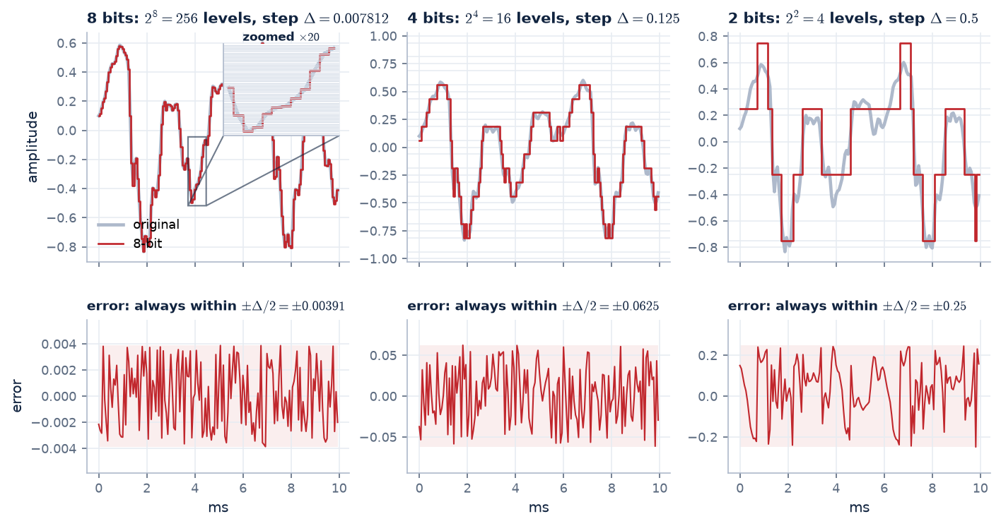
With \(b\) bits, each sample must be rounded to one of \(2^b\) levels. Fewer bits means fewer, coarser levels, and the rounding error becomes audible as a hiss, then a crackle, then distortion.
Figure 2. 10 ms of a vowel from our recording, rounded to 256, 16 and 4 levels. Top: the red staircase is what gets sent. At 8 bits the steps are too fine to see at full scale,
hence the \(\times 20\) zoom. Bottom: the quantisation error (sent minus original), each on its own scale. It always stays within half a step, \(\pm\Delta/2\), and every bit removed doubles that bound: \(\pm 0.004\) at 8 bits, \(\pm 0.06\) at 4 bits, \(\pm 0.25\) at 2 bits.
Each extra bit doubles the number of levels, which halves the step size and therefore halves the typical rounding error. Halving an amplitude is −6 dB, so:
$$\text{SNR} \approx 6.02\,b + 1.76\ \text{dB} \qquad\text{(full-scale sinusoid, uniform quantiser)}$$
every extra bit per sample buys about 6 dB of signal-to-noise ratio, and every bit removed costs about 6 dB. Derivation below.
Deriving \(\text{SNR} \approx 6.02\,b + 1.76\) dB
Step 1: the step size. A uniform quantiser with \(b\) bits splits the full range \([-1, 1)\) into \(2^b\) equal steps:
$$\Delta = \frac{2}{2^b} = 2^{1-b}$$
Step 2: the noise power. Rounding to the centre of a step leaves an error \(q\) that always lies within \(\pm\Delta/2\) (Figure 2, bottom row). When the step is small compared with the signal's
wiggles, every value in that interval is equally likely, so the error is uniformly distributed on \([-\Delta/2, \Delta/2]\) with density \(1/\Delta\). Its power is its mean square:
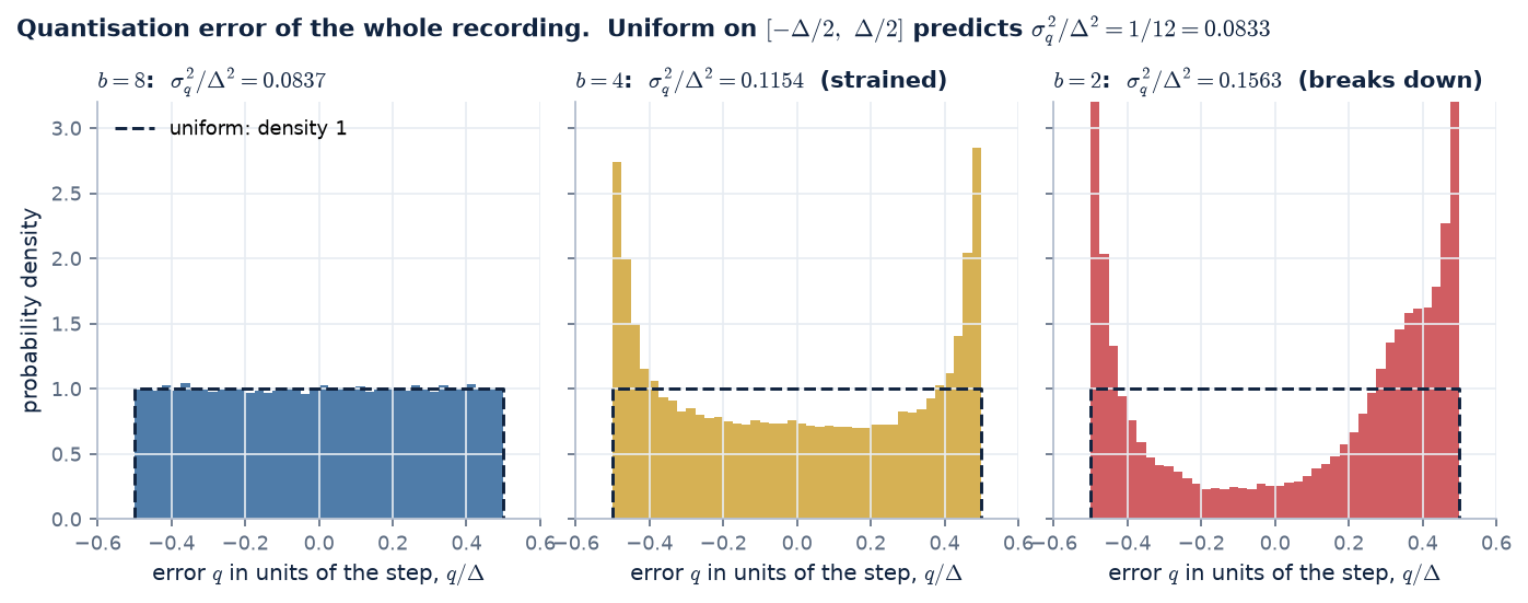
Figure 3. Checking the assumption on our recording. Each panel is a histogram of the error (sent minus original) of every sample, divided by the step \(\Delta\) so that all three share one axis.
The dashed box is the uniform density the derivation assumes. 8 bits: flat, and \(\sigma_q^2/\Delta^2 = 0.0837\), within 0.5 % of \(1/12\). 4 bits: the step (0.125) is now larger than many quiet samples, and errors
pile up near \(\pm\Delta/2\): a sample close to zero is always rounded to the first level, \(\pm\Delta/2\), so its error is nearly that level. The noise power is 38 % above \(\Delta^2/12\), which costs
1.4 dB (measured 8.6 dB, formula 10.0 dB). 2 bits: most of the signal fits inside one step and the error is mostly the signal itself, so the formula no longer applies.
Step 3: the signal power. A sinusoid that just fills the range, \(x(t) = \sin(\omega t)\), has power equal to its mean square, \(\overline{\sin^2} = \tfrac12\).
The 6.02 is “halving the step halves the error amplitude”, \(20\log_{10}2\). The 1.76 depends only on the signal's shape: it is the sinusoid's power of \(\tfrac12\) compared with the \(\tfrac{1}{12}\) in the noise.
For 16-bit audio this gives the familiar 98 dB, and for 8 bits about 50 dB. A quick simulation with a full-scale sinusoid gives 49.8 dB at 8 bits.
For any signal, Step 3 changes. A signal with rms value \(\sigma_x\) (full scale = 1) has power \(\sigma_x^2\), and the same algebra gives
The last term is the signal's level in dBFS, and it is negative. A full-scale sine has \(\sigma_x = 1/\sqrt2\) (−3.01 dB), which gives back 1.76. Our recording's rms level is only about −19 dBFS,
because speech has tall peaks and long quiet stretches. That predicts \(6.02 \times 8 + 4.77 - 18.9 \approx 34.0\) dB at 8 bits, and quantising the recording gives 34.0 dB. That is 15 dB worse than a sinusoid with the same number of bits.
The segmental SNR of Figure 6 is lower still (27.9 dB at 8 bits), because the quiet frames sit far below that average level. This penalty for quiet speech is exactly what \(\mu\)-law, in the next section, removes.
The uniform-error assumption fails when the signal is smaller than a few steps (Figure 3). At 1–2 bits, or for very quiet passages, the error becomes correlated with the signal and the formula is only a rough guide.
Knob 2: fewer samples per second (sampling rate)
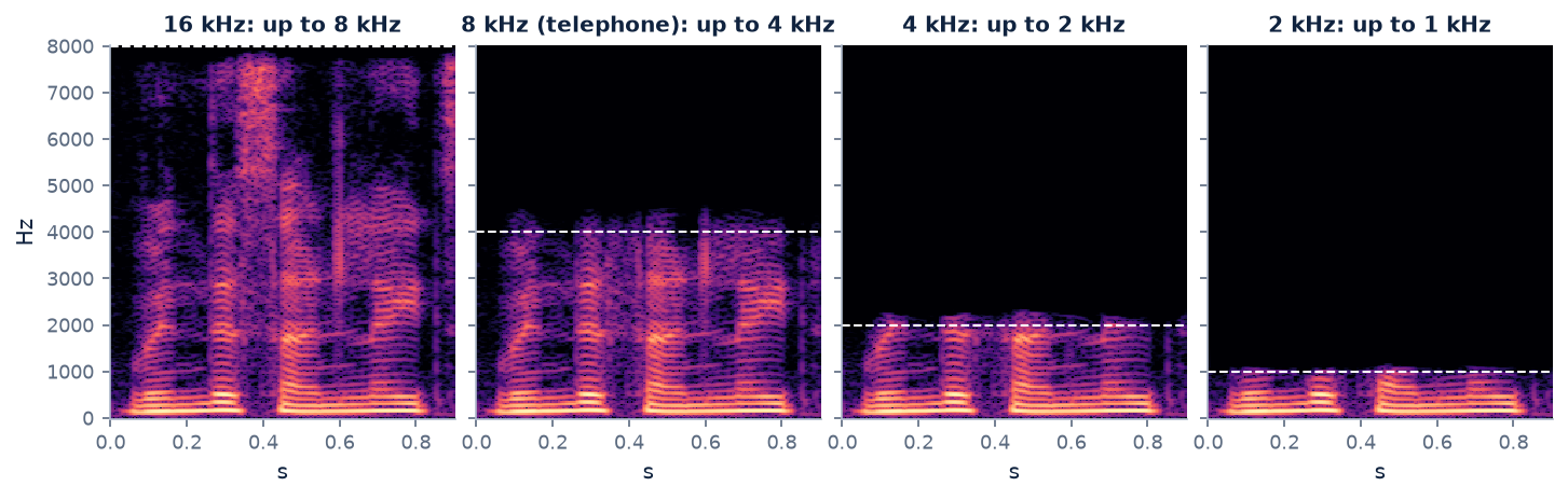
A signal sampled at \(f_s\) can only contain frequencies up to \(f_s/2\) (the Nyquist limit). Lowering \(f_s\) therefore cuts off the high frequencies: first the hiss of /s/ and /f/,
then the upper formants, until the speech sounds muffled, as if through a wall.
Figure 4. 0.9 s of our recording, including a fricative (the bright hiss high up near 0.4 s), at four sampling rates. At 8 kHz (the telephone) everything above 4 kHz is gone, and with it most of that hiss.
That is why “s” and “f” are hard to tell apart on the phone, and why people spell names as “S for Sierra”. At 2 kHz only the lowest formant survives.
Try both knobs
Choose a sampling rate, a number of bits and a quantiser. The recording is processed live in your browser. Watch the bit rate, and listen.
bit rate
Waveform, 20 ms: ■ original ■ processed
Spectrogram of the processed recording (0–8 kHz)
Listening examples
All examples on this page use one recording of an Indian-English speaker, at a range of bit rates. Segmental SNR (average SNR over 20 ms frames, higher is better) is given where the waveform is meant to match the original.
Original
256 kbit/s
16 kHz \(\times\) 16 bits, the reference.
16 kHz, 8 bits
128 kbit/s · segSNR 28.6 dB
Faint hiss in quiet parts.
16 kHz, 4 bits
64 kbit/s · segSNR 4.9 dB
Loud crackling noise riding on the speech.
16 kHz, 2 bits
32 kbit/s · segSNR -5.0 dB
Harsh distortion: four levels are not enough.
8 kHz, 16 bits
128 kbit/s
Telephone bandwidth: clean but duller; /s/ weakened.
4 kHz, 16 bits
64 kbit/s
Muffled: everything above 2 kHz is gone.
2 kHz, 16 bits
32 kbit/s
Only F1 survives: words very hard to follow.
8 kHz, 8 bits, uniform
64 kbit/s · segSNR 27.9 dB
64 kbit/s the naive way: audible noise floor.
Both knobs work up to a point, and then the price in quality becomes steep. To get from 256 down to 32 kbit/s you must either accept heavy noise (4 bits at 8 kHz) or a badly muffled voice (2 kHz sampling).
Neither knob knows anything about speech or about hearing.
03 · A first clever trick
\(\mu\)-law: spend the levels where the signal actually is.
A uniform quantiser treats every amplitude the same: its levels are evenly spaced from \(-1\) to \(+1\). Two facts about speech and hearing say that is a waste. We'll take them one at a time.
Fact 1 · Most speech samples are small
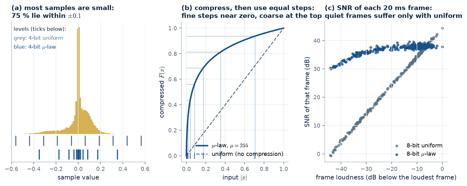
Make a histogram of every sample in our recording (Figure 5a). It is a tall, narrow spike around zero: 75 % of all samples lie within \(\pm 0.1\), a tenth of the full range.
Loud peaks are rare; quiet consonants, the tails of syllables, pauses and soft passages are common. Now look at where a 4-bit uniform quantiser puts its 16 levels (grey ticks under the histogram):
spread evenly across the whole range, so only 2 of the 16 levels fall where nearly all the samples are. Most of the levels sit out at large amplitudes that hardly ever occur.
Fact 2 · The ear judges noise relative to loudness
A uniform quantiser adds noise of the same absolute size (up to \(\pm\Delta/2\)) everywhere. In a loud vowel, a little hiss is masked by the speech. In a quiet consonant or a soft-spoken word, the
same hiss is relatively much bigger and clearly audible. What matters to a listener is roughly the ratio of signal to noise in each moment, not the absolute noise level. (This is the same
relative sensitivity that makes us measure sound in decibels.)
The fix · fine steps for small values, coarse steps for big ones
Both facts point the same way: put the quantiser levels close together near zero and further apart for large amplitudes. Ideally the step size grows in proportion to the amplitude,
so the noise stays a fixed fraction of the signal. That is a logarithmic spacing. The neat trick is that we don't need a new quantiser to get it. We bend the signal first and keep the simple uniform one:
1 · compress
Pass each sample through a log-like curve \(F(x)\). Small values are stretched apart, large values squeezed together.
2 · quantise uniformly
Round \(F(x)\) to \(b\) bits with ordinary equal steps, and send those bits.
3 · expand
The decoder applies the inverse curve \(F^{-1}\), turning the equal steps back into small steps near zero and big steps for loud values.
The curve used in North American and Japanese telephony is \(\mu\)-law:
$$F(x) = \operatorname{sgn}(x)\,\frac{\ln(1 + \mu|x|)}{\ln(1 + \mu)}, \qquad F^{-1}(y) = \operatorname{sgn}(y)\,\frac{(1+\mu)^{|y|} - 1}{\mu}, \qquad \mu = 255,\ |x| \le 1$$
\(\mu\) sets how strongly the curve bends: \(\mu \to 0\) gives a straight line (plain uniform quantisation); \(\mu = 255\) stretches the bottom of the range enormously. For \(\mu|x| \gg 1\) the curve is logarithmic, giving the constant relative step we wanted; near zero it becomes linear, so it stays well-behaved at silence.
Figure 5. \(\mu\)-law, step by step, on our recording at 8 kHz. (a) The sample values pile up near zero. Uniform levels (grey) ignore that; \(\mu\)-law levels (blue) crowd into the busy region.
(b) The compression curve: equally spaced levels on the vertical (compressed) axis land at very unequal spacings on the input axis, tiny near zero and large near \(\pm 1\).
(c) The payoff, measured on every 20 ms frame: with 8-bit uniform PCM the SNR falls one-for-one as the frame gets quieter (a frame 40 dB down has almost no SNR left). With 8-bit \(\mu\)-law
the SNR stays above about 30 dB (mostly 35–39 dB) for loud and quiet frames alike.
Try it: bend the levels yourself
The histogram of our recording's samples, with the quantiser's levels drawn on top. Raise \(\mu\) from 0 (uniform) and watch the levels migrate towards zero, where the samples are.
bits:
Sample histogram (zoomed to \(\pm 0.5\)) with the quantiser's reconstruction levels (blue lines)
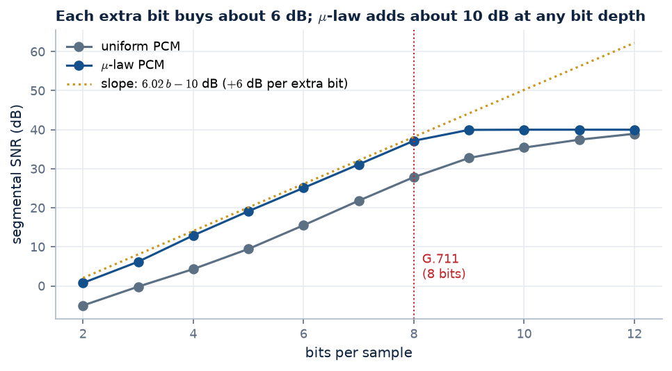
Figure 6. The overall effect across bit depths (segmental SNR, our recording at 8 kHz). Both lines climb about 6 dB per bit, but \(\mu\)-law sits about 10 dB higher: 8-bit \(\mu\)-law \(\approx\) 10-bit uniform,
roughly 2 bits per sample saved for free. (The curves flatten at the top only because segmental SNR is conventionally capped at 40 dB per frame.)
This is G.711 (1972): \(8000 \times 8\) bits/s with \(\mu\)-law (North America, Japan) or the very similar A-law (Europe, India and most of the world), giving 64 kbit/s.
In the standard the smooth curve is approximated by 8 straight-line segments per polarity, cheap to build in 1970s hardware. G.711 has been the backbone of digital telephone networks for half a century, and it
is the reference that “toll quality” is measured against. Compare 8-bit uniform with 8-bit \(\mu\)-law in the listening grid, and 4-bit uniform with 4-bit \(\mu\)-law in section 05: same bit rate, very different noise.
Why \(\mu = 255\)? An engineering compromise
\(\mu\) is a dial between two goals that pull against each other. A telephone network has to serve soft talkers and loud talkers, on short and long lines. Their levels differ by
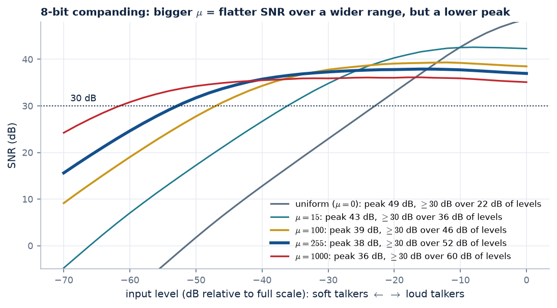
tens of dB, and every one of them should get a decent SNR. Measure the SNR of an 8-bit coder as the input level is swept from very soft to full scale (Figure 7):
Figure 7. 8-bit coding of a speech-like (Laplacian) signal at different input levels. Uniform (\(\mu = 0\)) is superb for loud talkers but falls one dB per dB as they get softer, staying above
30 dB for only 22 dB of levels. Raising \(\mu\) flattens the curve, widening the usable range (\(\mu = 255\): 52 dB), but it lowers the ceiling (38 dB instead of 49). \(\mu = 1000\) is flatter still, at an even lower peak.
So the choice of \(\mu\) answers a practical question: how wide a range of talker levels must be served, and how much peak quality are we willing to give up for it? The history, as usually told:
1957: the family. Bernard Smith at Bell Labs analysed “instantaneous companding” and formulated the logarithmic \(\mu\)-law curves, showing how \(\mu\) trades dynamic range against peak SNR, the trade-off of Figure 7.
1962: \(\mu = 100\), 7 bits. The first commercial digital telephone system, Bell's T1 carrier, coded speech with 7-bit \(\mu\)-law and \(\mu = 100\).
Around 1970: \(\mu = 255\), 8 bits. The next generation of equipment moved to 8 bits. With one more bit, a stronger curve could keep an SNR in the mid-30s of dB across the full range of talker levels found in the network.
There was also a hardware reason. The smooth curve is built from 8 straight-line segments per polarity, each twice as long as the one before, and with \(\mu = 2^8 - 1 = 255\) the segment boundaries fall on
binary-friendly values. A logarithm could then be computed with simple 1970s digital logic: a 3-bit “which segment” (exponent) and a 4-bit “where in the segment” (mantissa), a tiny floating-point number.
A-law. European engineers chose a slightly different curve with \(A = 87.6\), also built from straight segments. It is very close to \(\mu\)-law in performance.
Note what drove the choice: measured talker levels, SNR targets and what hardware could build cheaply. These were engineering numbers, checked against the listening experience of telephone engineers.
Formal, large-scale listening tests with panels of ordinary listeners became the centrepiece of codec selection later.
Is \(\mu\)-law perfectly invertible?
The curve, yes. The coder, no. \(F(x)\) is strictly increasing, and \(F^{-1}\) undoes it exactly: compressing and expanding a million random values reproduces them to within \(10^{-15}\) (floating-point rounding).
But the decoder computes \(\hat{x} = F^{-1}\bigl(Q(F(x))\bigr)\), and the expander cannot undo the rounding \(Q\) in the middle: every input within one step maps to the same 8-bit code. \(\mu\)-law is lossy; it just
places the loss cleverly. At 8 bits and \(\mu = 255\) the steps (in \(x\)) range from 0.00017 near zero to 0.042 near full scale, about 243 times wider. Near zero that is as fine as a uniform quantiser with about 13.5 bits
(G.711 \(\mu\)-law is indeed specified as an 8-bit code for a 14-bit linear signal), while for \(|x| > 0.1\) the error never exceeds about 2.3 % of the value.
A useful bonus: decoding and then re-encoding gives back exactly the same codes, because every decoded value sits on a reconstruction level, inside its own rounding interval. A call that passes through several
\(\mu\)-law encode/decode stages in the network therefore suffers no extra loss after the first one.
\(\mu\)-law doesn't use fewer bits. It spends the same bits more wisely, matching the quantiser to how speech amplitudes are distributed and to how loudly we perceive noise.
It is the first example on this page of a theme that runs to the end: the more a coder knows about speech and hearing, the fewer bits it needs.
04 · Can we do better?
A waveform coder treats every sample as a surprise. Speech isn't.
PCM, even with \(\mu\)-law, sends every sample in full, as if it were completely new information. But module 4 showed that speech is highly predictable: a weighted sum of the last 10 samples
guesses the next one very well. On this recording at 8 kHz, a 10th-order predictor leaves an error 13 dB weaker than the signal itself. That redundancy is pure waste for a waveform coder.
Recap: prediction gain
The prediction gain compares the energy of the signal with the energy of the error a predictor leaves:
13 dB means the error carries only about 5 % of the signal's energy. Why it converts into bits: a quantiser's noise depends on its step size, and the step needed depends on how big the values to be coded are.
Values about \(10^{13/20} \approx 4.5\) times smaller in amplitude need about \(\log_2 4.5 \approx 2.2\) fewer bits for the same noise.
(Full explanation, with more examples and what the number depends on: module 4, “What is prediction gain?”.)
Combine that with the 6-dB-per-bit rule from section 02:
$$\text{bits saved per sample} \approx \frac{\text{prediction gain (dB)}}{6.02\ \text{dB/bit}} = \frac{13.3}{6.02} \approx 2.2\ \text{bits/sample} \;\Rightarrow\; \approx 18\ \text{kbit/s saved at } 8\ \text{kHz}$$
And there is more structure to exploit than that. Module 5 showed that speech is a source (pulses or noise) through a filter (a few formants), both changing slowly, every 10–20 ms. If the receiver
already knows that model, maybe we only need to send its settings. The next three sections climb that ladder of ideas, one trick at a time.
05 · Trick 2: code only the surprise
Predictive coding (DPCM / ADPCM).
Don't send the sample. Send the prediction error, the part the receiver couldn't have guessed. Because the error is much smaller than the signal, the same quantiser step gives far
less noise, or the same noise needs fewer bits.
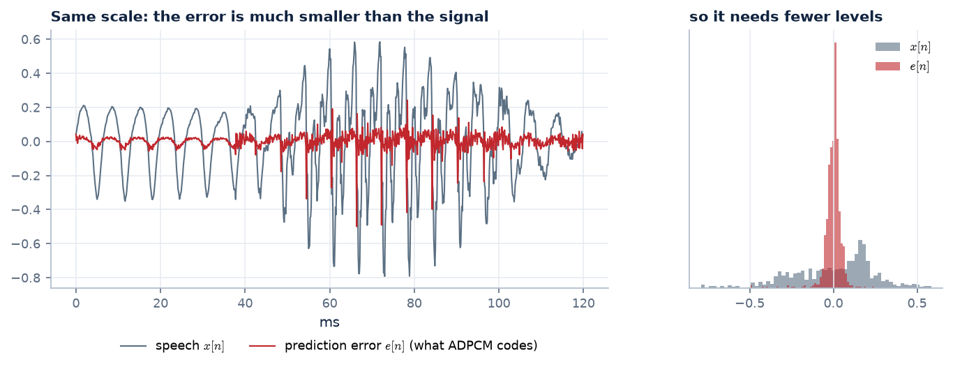
Figure 8. 120 ms of speech (grey) and the error left by a 10-weight predictor (red), on the same scale. The error is much smaller and its values are concentrated near zero, so fewer quantiser levels cover it.
$$e[n] = x[n] - \hat x[n], \qquad \hat e[n] = Q\bigl(e[n]\bigr), \qquad \tilde x[n] = \hat x[n] + \hat e[n] \;\Rightarrow\; \tilde x[n] - x[n] = \hat e[n] - e[n]$$
\(\hat x[n] = \sum_k a_k\,\tilde x[n-k]\) is the prediction, made from past decoded samples \(\tilde x\). The last identity is the point of the design: the decoder's error is exactly the quantiser's error for that sample, so errors never pile up.
Figure 9. DPCM. The encoder subtracts a prediction \(\hat x[n]\), quantises the small error \(e[n]\) and sends \(\hat e[n]\). It also rebuilds the decoded sample \(\tilde x[n]\) exactly as the decoder will, and feeds that, not the original, to its predictor.
Both sides therefore make exactly the same prediction from the same numbers. “Adaptive” DPCM (ADPCM) also re-fits the predictor and the
quantiser's step size as the speech changes, again only from already-decoded data, so no extra side information needs to be sent.
What exactly is the predictor?
It is linear prediction, the same as in modules 4–5: a weighted sum of the last \(p\) samples,
Two things differ from the LP analysis of module 4. First, it runs on the decoded samples \(\tilde x\), not the originals, so the encoder and the decoder make the same guess
(the DPCM diagram above). Second, the weights \(a_k\) have to reach the decoder somehow. There are three ways to arrange that:
approach
where the weights come from
sent as side information?
example
Fixed (plain DPCM)
Designed once from the average statistics of speech and never changed. The simplest is first order,
\(\hat x[n] = 0.9\,\tilde x[n-1]\): neighbouring samples of 8 kHz speech are highly correlated.
no
early DPCM systems
Forward adaptive
The encoder runs LPC (Levinson–Durbin) on each frame of the original speech, quantises the weights and sends them, like the
vocoder's 45 filter bits in section 06.
yes, every frame
adaptive predictive coding (APC)
Backward adaptive
Encoder and decoder both re-estimate the weights from the past decoded signal, with the same rule, so they arrive at the same values
independently.
no
ADPCM (G.726, and ours)
The “A” in ADPCM can adapt two things, and usually both: the quantiser step (Jayant's rule: after a large error code, make the step bigger; after a small one,
smaller) and the predictor weights, which follow the speech from one sound to the next.
Our coder (adpcm() in codecs/make_assets.py): an order-10 predictor. Every 10 ms, both sides run Levinson–Durbin on the last
256 decoded samples (32 ms) to get fresh weights; the step follows Jayant's multipliers. Only the error codes are transmitted. The “adaptive step, no prediction”
clips below switch the predictor off (\(\hat x[n] = 0\)), so you can hear what prediction alone adds.
G.726 does not refit on blocks. Its predictor has 2 feedback (pole) and 6 feed-forward (zero) weights, and nudges them a tiny step after every sample with a
simple gradient rule (a sign–sign LMS update).
In one line: the predictor is an LP filter, and in ADPCM its coefficients are learned from the decoded signal by encoder and decoder in step, instead of being transmitted.
Listen to four coders at the same 32 kbit/s (\(8000 \times 4\) bits/s), each adding one idea:
4-bit PCM baseline
32 kbit/s · segSNR 4.3 dB
No tricks: noise everywhere.
4-bit \(\mu\)-law + companding
32 kbit/s · segSNR 12.9 dB
Levels spread to match loudness.
4-bit adaptive step + adaptation
32 kbit/s · segSNR 19.3 dB
Step size follows the loudness, no prediction yet.
4-bit ADPCM + prediction
32 kbit/s · segSNR 23.7 dB
Adaptive step + 10-weight predictor: code only the error.
3-bit ADPCM
24 kbit/s · segSNR 20.1 dB
24 kbit/s: noisier but clearly usable.
2-bit ADPCM
16 kbit/s · segSNR 15.3 dB
16 kbit/s: a 2-bit coder that still carries the speech.
Prediction plus an adaptive step turns an unusable 4-bit coder (segmental SNR about 4 dB) into one that comes within about 4 dB of 8-bit uniform PCM, at half the bit rate. This is the idea of G.726 ADPCM (32 kbit/s, also 16–40),
long used in cordless phones (DECT) and on international trunk lines. Our implementation is simpler than the standard, and its prediction delivers about 4 dB of the theoretical 13. The gap is the last point in module 4's list: the decoder can only refit the predictor from
decoded, noisy samples (with 4 bits, those are quite noisy), and the ideal 13 dB was measured with the weights fitted to the clean original. The principle is the same.
How does it start? The first sample
The very first prediction has no past to use. Encoder and decoder simply agree on a starting state, usually empty memory: all decoded samples before the start count as zero. Then
The first sample is coded as its own “error” through the same quantiser, and nothing extra is sent. For a \(p\)-th order predictor, the first \(p\) samples are predicted from partial history padded with zeros. This is harmless for three reasons:
Speech usually starts in silence, where predicting 0 is correct.
The loop is closed. The encoder predicts from \(\tilde x\), the decoded signal, so it tracks the decoder's state exactly from \(n = 0\). A crude start costs a little quality for a few milliseconds and never accumulates: \(\tilde x[n] - x[n] = \hat e[n] - e[n]\) holds for every \(n\).
The real start-up cost is the step size. ADPCM's adaptive step also starts from an agreed value. If speech begins loudly, the first few samples overload the quantiser until the step has grown, which takes a few milliseconds. Standards such as G.726 define exact reset values so every implementation starts identically.
When the state is sent explicitly. Block-based ADPCM files (IMA ADPCM in WAV files, for example) start every block of a few hundred samples with a small header: the first sample at full 16-bit precision and the starting step size.
A player can then begin decoding at any block. On noisy channels the same idea gives robustness: a corrupted bit makes the decoder's memory differ from the encoder's, and periodic resets, or a slight
“leak” that makes the decoder gradually forget old values, bring the two back into step.
Our implementation (adpcm() in codecs/make_assets.py) predicts 0 until it has \(p\) samples, and uses no predictor for the first 256 samples (32 ms) because its first fit needs that much decoded history. The recording begins in near-silence, so this start-up is inaudible.
06 · Trick 3: send the model, not the waveform
The LPC vocoder: 57 bits every 20 ms.
ADPCM still sends something for every single sample. Module 5 suggested a far more radical idea: speech = source through an all-pole filter, and both change slowly. So, every 20 ms,
the encoder just measures the model's settings and sends those. The decoder, which knows the model, rebuilds speech from them: pulses at the right pitch (or noise), through the right filter, at the right loudness.
Bit budget per 20 ms frame (our implementation, 8 kHz, order 10)
parameter
what it describes
bits
10 reflection coefficients (as log-area ratios)
the vocal-tract filter: formants
45
pitch period
the buzz rate, 60–400 Hz on a log scale
6
voiced / unvoiced flag
pulses or noise?
1
gain
loudness (dB)
5
total per frame · \(\times\, 50\) frames per second
57 bits → 2 850 bit/s
That is 90 times less than the 256 kbit/s original, and 11 times less than ADPCM. Two small tricks make the filter cheap to send:
Send reflection coefficients, not the weights. The predictor weights \(a_k\) are fragile: a tiny rounding error can push a pole outside the unit circle and make the decoder's filter unstable (module 5).
The equivalent reflection coefficients \(k_i\) (one per joint in the tube model) are always between \(-1\) and \(+1\), and the filter is stable as long as they stay there. So they can be rounded safely.
Quantise them on a warped scale. The important values of \(k\) crowd near \(\pm 1\), so they are quantised as log-area ratios, \(\ln\frac{1+k}{1-k}\) (literally the log of the area ratio between neighbouring tube sections), which spreads them out. Fewer bits go to the higher, less important coefficients.
Original
256 kbit/s
256 kbit/s.
LPC vocoder, exact parameters
unquantised parameters
Model only: pulses or noise through the measured filter.
LPC vocoder, 57 bits / 20 ms
2.85 kbit/s
Parameters rounded to the bit budget above.
The words are clear and the voice is recognisably the same speaker, but it is unmistakably robotic: the real glottal waveform has been replaced by clicks, and voiced/unvoiced is a hard switch. This is
“synthetic quality”, the sound of LPC-10 (2.4 kbit/s, US Federal Standard 1015, 1984), of military secure telephones, and of Texas Instruments' Speak & Spell.
Note that removing the quantisation (left) changes little: the loss of quality comes from the model's crude source, not from the rounding.
Check your understanding
1. A podcast is recorded at 48 kHz, 24 bits, stereo. What is its raw bit rate, and how big is one hour?
\(48\,000 \times 24 \times 2 = 2304\) kbit/s; one hour is \(2.304 \times 10^6 \times 3600 / 8 \approx 1.04\) GB. A typical speech podcast is distributed at 64–128 kbit/s, 20–35 times smaller.
2. Why does ADPCM's predictor use the decoded samples rather than the original ones?
The decoder only has the decoded samples. If the encoder predicted from the originals, the two predictions would differ by the quantisation errors, which would accumulate at the decoder and drift away from the speech. Predicting from decoded samples keeps both sides in lock-step.
3. The LPC vocoder's SNR is not shown. Why is SNR meaningless for it?
It makes no attempt to reproduce the waveform: its pulses are at the right rate but not at the original's exact instants, and its noise is a different random signal. The output can sound similar while being completely uncorrelated sample by sample, so its SNR would be near or below 0 dB.
4. Why are reflection coefficients (or log-area ratios) transmitted instead of the predictor weights?
Rounding the weights can move a pole outside the unit circle and make the decoder's filter unstable. Reflection coefficients guarantee stability as long as each stays inside \((-1, 1)\), which is easy to enforce after quantisation, and their sensitivity is better handled on the log-area-ratio scale.
5. Telephone speech is band-limited to 3.4 kHz. Which sounds suffer most, and how do listeners cope?
Fricatives such as /s/, /f/ and /θ/, whose energy lies mostly above 4 kHz, become hard to tell apart. Listeners lean on context, and spelling alphabets (“S for Sierra”) exist for exactly this reason. Wideband (“HD voice”) codecs at 16 kHz bring these cues back.