Seeing Sound: the Spectrogram

01 · Why we need it

One picture for when and which frequency.

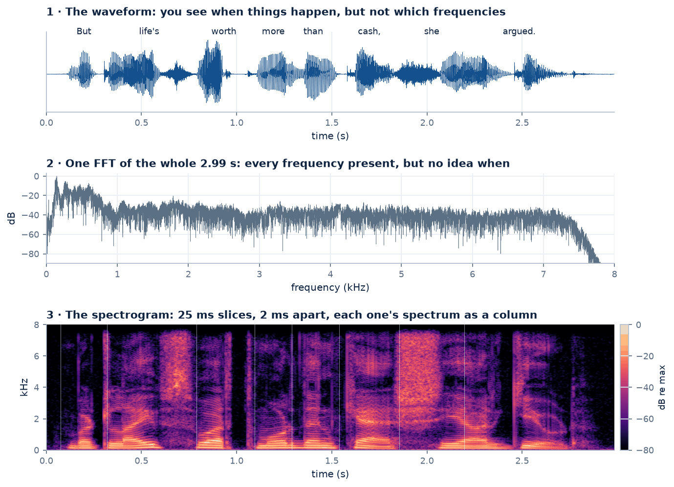
Here is one sentence, “But life's worth more than cash, she argued.”, 2.99 s long, sampled at 16 kHz. Look at it three ways.

The ksp sentence as a waveform, as one whole-utterance spectrum, and as a spectrogram — **Figure 1.** The same 47761 samples, three ways. **Top:** the waveform shows loud and quiet stretches, so you can find the words, but not which frequencies are present. **Middle:** one FFT of the whole sentence has a frequency point every 0.335 Hz, beautifully detailed, but it mixes the /s/, the vowels and the pauses into one curve: there is no “when” left. (The fall above 7.5 kHz is the recording's anti-aliasing filter.) **Bottom:** the spectrogram keeps both. The hiss of /s/ in “life's” and of /ʃ/ in “cash, she” shows as tall noisy blocks, the vowels as stacks of horizontal lines low down.

The waveform and the whole-signal spectrum are two extremes. One has perfect time detail and no frequency axis; the other has perfect frequency detail and no time axis. Speech needs something in between, because speech changes all the time. Over the whole ksp recording set (1132 sentences, 35965 phones), the median phone lasts 80 ms, and 80 % of phones last between 25 and 155 ms. Inside a phone, the vocal folds open and close every few milliseconds. A spectrum of the whole sentence averages all of that away.

Cut the signal into short, overlapping slices, short enough that the sound is roughly steady inside each one (a few to a few tens of milliseconds), take the spectrum of every slice, and stand the spectra side by side. That is the short-time Fourier transform (STFT), and its magnitude, drawn as an image, is the spectrogram.

A spectrogram is like a musical score that writes itself: time left to right, pitch bottom to top, and loudness as darkness or colour. The difference is that it shows every frequency, not just the notes, so it also draws noises, bursts and the resonances of the vocal tract.

The idea is older than digital computers. In 1946 Koenig, Dunn and Lacy at Bell Telephone Laboratories described the sound spectrograph, which scanned a recording with a tunable band-pass filter and burnt the output onto paper. A year later Potter, Kopp and Green published Visible Speech, a book that taught people to read words from these pictures. Every spectrogram on this page is computed the digital way, with the FFT.

02 · The STFT, step by step

Frame, window, FFT, magnitude, stack.

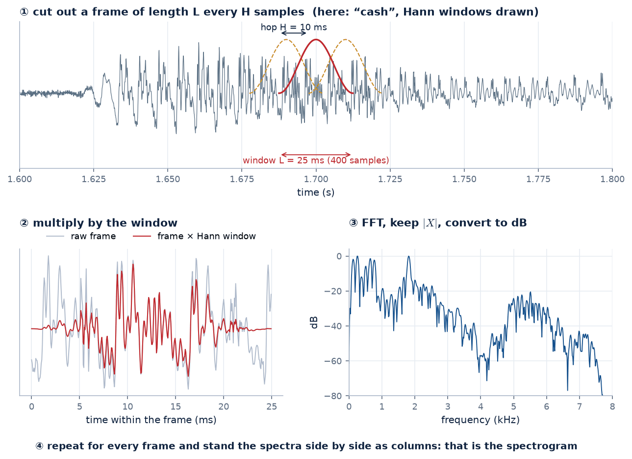
The recipe has five steps, and three numbers control it.

The STFT steps on a vowel: framing with Hann windows, the windowed frame, and its spectrum in dB — **Figure 2.** The steps on the vowel of “cash”. ① Choose a frame of $L$ samples, then move along by a *hop* of $H$ samples to the next one (here 25 ms and 10 ms, so neighbouring frames overlap by 60 %). ② Multiply the frame by a smooth window that falls to zero at both ends. ③ Take the FFT and keep the magnitude, in dB. ④ Do this for every frame and place the spectra side by side as columns.

Written as one formula, the STFT of a signal $x[n]$ with a window $w[n]$ of length $L$ is

$$X[m,k] \;=\; \sum_{n} x[n]\; w[n - mH]\; e^{-j 2\pi k n / N}, \qquad k = 0, 1, \dots, N-1$$ $m$ numbers the frames (frame $m$ starts at sample $mH$), $k$ numbers the frequency bins, and $N \ge L$ is the FFT size. The window is zero outside $0 \le n - mH < L$, so each $X[m,\cdot]$ only sees one slice. Written this way the phase is measured from the start of the signal; many libraries put $n - mH$ in the exponent instead, which changes the phase of $X$ but not $|X|$.

Frame $m$ sits at time $t_m = mH/f_s$ and bin $k$ at frequency $f_k = k f_s / N$. The spectrogram is the magnitude, usually squared and in decibels:

$$S_{\text{dB}}[m,k] = 20\log_{10}\bigl|X[m,k]\bigr| \;=\; 10\log_{10}\bigl|X[m,k]\bigr|^2$$ The phase $\angle X[m,k]$ is thrown away for the picture. Section 6 shows what that costs when we want the sound back.

The three numbers: $L$, $H$ and $N$

symbol	name	what it controls	typical for speech at 16 kHz
$L$	window length	how long a slice the analysis “sees”, and so the trade-off between time detail and frequency detail (section 4)	5–40 ms (80–640 samples)
$H$	hop	how often a column is computed; it sets the picture's time sampling but not its time resolution	1–10 ms, usually $L/4$ to $L/2$
$N$	FFT size	how many frequency points are drawn: the bin spacing is $f_s/N$	the next power of two $\ge L$, e.g. 512

Bin spacing is not resolution

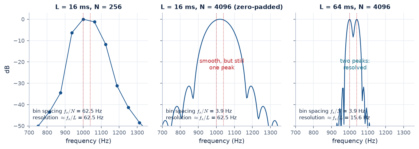
A common confusion: if $N$ sets the bin spacing, why not use a huge FFT and get fine frequency detail for free? You can pad the frame with zeros up to any $N$. But the zeros add no information. They only interpolate between the points you already had. The ability to tell two nearby frequencies apart, the resolution, is set by how long a stretch of signal you looked at: roughly $f_s/L$ hertz, times a factor of 1–2 that depends on the window.

Two tones 40 Hz apart: a short window with and without zero-padding, and a long window — **Figure 3.** A synthetic signal: two equal tones at 1000 and 1040 Hz, Hann window. **Left:** a 16 ms window and a 256-point FFT gives one point every 62.5 Hz. **Middle:** the same 16 ms padded to 4096 points draws a smooth curve, but still one lump: zero-padding only interpolated it. **Right:** a 64 ms window separates the two tones. Only a longer look resolves them.

The STFT machine

Drag the time slider, or press run: the red window slides along the sentence, and every 2 ms its spectrum is painted as one more column of the spectrogram.

window length: window:

time:

① the sentence and the current window (red)

② the frame (grey) and the windowed frame (red)

③ its spectrum, dB re the loudest frame of the sentence

④ the spectrogram so far (80 dB range)

Park the slider in the /s/ of “life's” (about 0.70 s) and then in the vowel of “cash” (about 1.70 s). The /s/ spectrum is a ragged plateau above 3–4 kHz; the vowel spectrum is a comb of harmonics with humps (formants). Switch to the rectangular window in the vowel and watch the gaps between harmonics fill up: that is leakage, the topic of the next section.

03 · Windows and leakage

Why not just cut the signal with scissors?

Cutting a frame out with no window at all is the same as multiplying by a rectangular window: 1 inside, 0 outside. Multiplying in time is convolving in frequency, so every spectral line in the frame is replaced by a copy of the window's own spectrum. A sharp-edged window has a spectrum with tall side lobes, so energy from a strong component spills, or leaks, into bins far away and can bury weak components there. A window that tapers smoothly to zero has much lower side lobes, at the price of a wider main lobe, which blurs nearby frequencies together.

$$w_{\text{Hann}}[n] = 0.5 - 0.5\cos\frac{2\pi n}{L}, \qquad w_{\text{Hamming}}[n] = 0.54 - 0.46\cos\frac{2\pi n}{L}, \qquad 0 \le n < L$$ Hamming is a Hann window lifted onto a small pedestal (it ends at 0.08, not 0). The weights are chosen to cancel the first side lobe, which lowers the highest side lobe but leaves a step at the edges, so its far side lobes decay slowly. (With $L-1$ in the denominator instead of $L$ these are the symmetric versions; section 6 explains why the difference matters.)

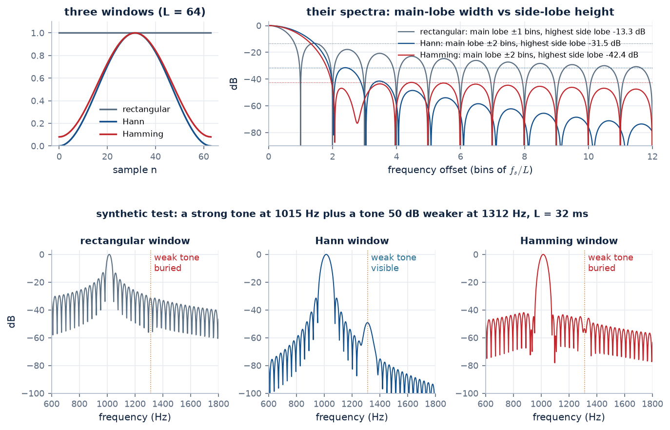
Rectangular, Hann and Hamming windows, their spectra, and a two-tone leakage test — **Figure 4.** **Top:** the three windows and their spectra, with frequency in bins of $f_s/L$. **Bottom:** a synthetic test with a strong tone at 1015 Hz and one 50 dB weaker at 1312 Hz, 9.5 bins away, analysed over 32 ms. With the rectangular window the strong tone's leakage near the weak one is about −29.3 dB and hides it. With Hann the leakage there has fallen to about −61.5 dB and the weak tone stands out. Hamming has the lowest *highest* side lobe, but its side lobes stay near −47.9 dB far from the peak, which is just enough to swamp a tone at −50 dB.

window	highest side lobe	main lobe, null to null	main lobe, −6 dB width	far side lobes fall at
rectangular	−13.3 dB	2 bins	1.21 bins	−6 dB per octave
Hann	−31.5 dB	4.1 bins	2.04 bins	−18 dB per octave
Hamming	−42.4 dB	4.1 bins	1.84 bins	−6 dB per octave

Measured here on 64-sample symmetric windows (hence null-to-null widths slightly above 4 bins). Harris (1978) gives −13, −31 and −43 dB for long windows; the roll-off rates are his. One bin is $f_s/L$: 40 Hz for a 25 ms window at 16 kHz.

For speech, Hann and Hamming are both fine and both common: classic speech recognisers used Hamming (HTK, for example), while many newer toolkits default to Hann. The rectangular window is almost never right for a spectrogram. The −6 dB main-lobe width is a fair measure of resolution: with a Hann window two equal components need to be about 2 bins, $2f_s/L$, apart to show as two peaks.

A window trades leakage (side lobes, which let loud parts spill into quiet regions) against blur (main-lobe width, which merges close frequencies). In a speech spectrogram, where loud low harmonics sit next to formants 40–60 dB weaker, low side lobes matter more than the last bit of sharpness, so we always taper.

04 · Wideband or narrowband

You cannot have sharp time and sharp frequency at once.

A window of $L$ samples lasts $\Delta t \approx L/f_s$ seconds and resolves about $\Delta f \approx f_s/L$ hertz. Their product is a constant: make the window shorter for better timing and the frequency detail gets coarser by the same factor. This is a property of the Fourier transform itself (Gabor's form of the uncertainty principle), not of the FFT:

$$\Delta t \cdot \Delta f \approx \frac{L}{f_s}\cdot\frac{f_s}{L} = 1, \qquad\text{and strictly}\quad \sigma_t\,\sigma_f \ge \frac{1}{4\pi}$$ $\sigma_t$ and $\sigma_f$ are the rms durations and bandwidths of the window; a Gaussian window reaches the bound. The exact constant depends on how widths are defined, the trade-off does not.

For voiced speech the natural ruler is the pitch period $T_0 = 1/F_0$, the time between glottal pulses. From the corpus pitch marks inside the vowels of our sentence, ksp's median period is 7.4 ms, so $F_0 \approx$ 134 Hz (80 % of the 119 periods lie between 109 and 152 Hz). Compare the window with that period:

Wideband: $L < T_0$

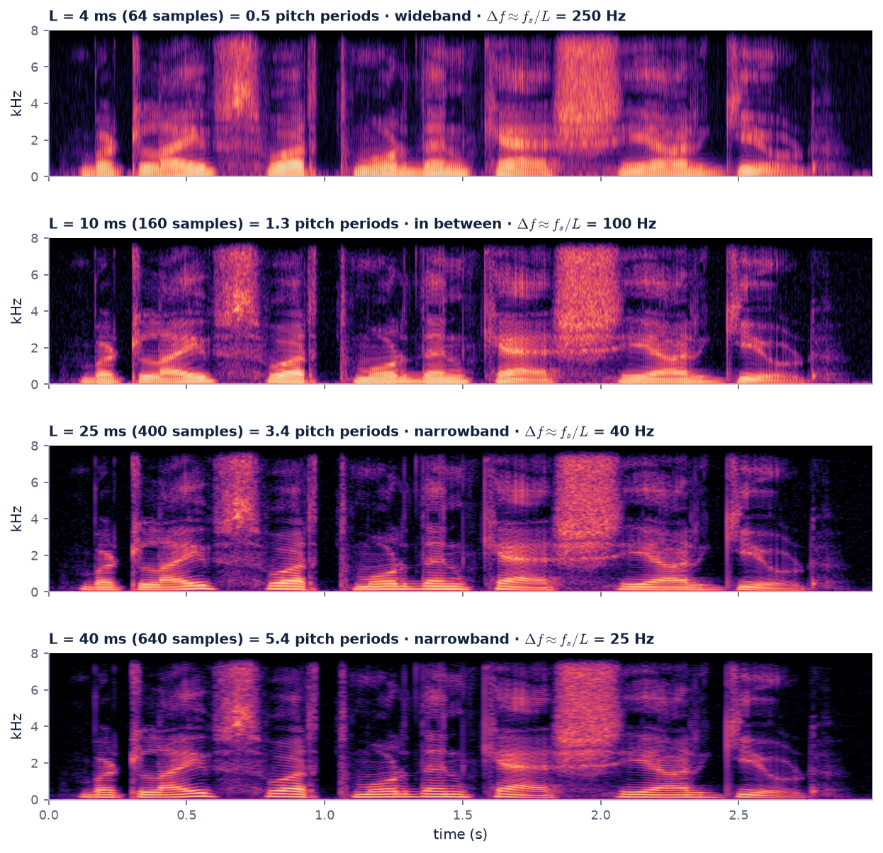
A 3–5 ms window sees less than one period. Each frame either contains a glottal pulse or does not, so the picture shows vertical striations, one per pulse. Its frequency blur (about 250 Hz for 4 ms) smears the harmonics together into broad formant bands. Best for formants, bursts and timing.

Narrowband: $L \gtrsim 2\text{–}3\,T_0$

A 25–40 ms window spans several periods. The periodicity shows up in frequency as horizontal harmonics at $F_0, 2F_0, 3F_0, \dots$, each about $f_s/L$ = 25–40 Hz wide. Timing blurs over the window. Best for pitch and intonation.

The sentence with 4, 10, 25 and 40 ms windows — **Figure 5.** The same sentence with Hann windows of 4, 10, 25 and 40 ms (0.5, 1.3, 3.4 and 5.4 pitch periods of 7.4 ms). At 4 ms the vowels are vertical stripes under dark formant bands and every burst is a crisp vertical line. At 25–40 ms the vowels turn into stacks of harmonic lines and the bursts smear sideways. 10 ms, about one period, shows neither pattern cleanly.

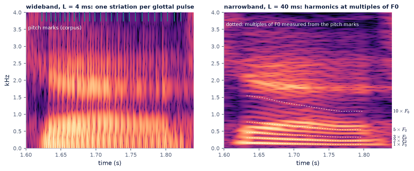
Close-up of the vowel in cash: striations with a 4 ms window and harmonics with a 40 ms window — **Figure 6.** A close-up of the vowel /æ/ in “cash”. **Left (4 ms):** the vertical striations line up with the corpus pitch marks (ticks at the top), one per glottal closure. **Right (40 ms):** the harmonics follow the dotted lines at multiples of the $F_0$ measured from those pitch marks. Pitch falls through this vowel, from about 152 to 108 Hz, so every harmonic slopes down, and the tenth falls ten times as far as the first. That fast change is also why high harmonics blur in a long window: the pitch moves during the 40 ms the window looks at.

Slide the window length

window length $L$:

Start at 4 ms in the “cash” zoom and count the striations in 50 ms: there should be about $50/7.4 \approx 7$. Then slide slowly up. Near 8–12 ms (one period) the stripes fade and the harmonics have not yet appeared. By 25 ms the harmonics are clear. A child or many female voices, with $F_0$ of 200–300 Hz, would need a window of about 3 ms or less for a true wideband view.

Phoneticians usually read wideband spectrograms, because formants and the timing of bursts and closures carry most of the phonetic information. The classic analogue sound spectrograph offered exactly these two choices: a wide (300 Hz) and a narrow (45 Hz) analysing filter. Speech recognisers and neural models use a compromise, typically 25 ms (section 8).

05 · Decibels and colour

How the numbers become a picture.

A spectrogram is a grid of numbers, $|X[m,k]|$. To draw it we choose a scale (linear or decibels), a range (which values map to the darkest and brightest colours) and a colour map. Each choice changes what you can see.

Linear or dB, and how many dB

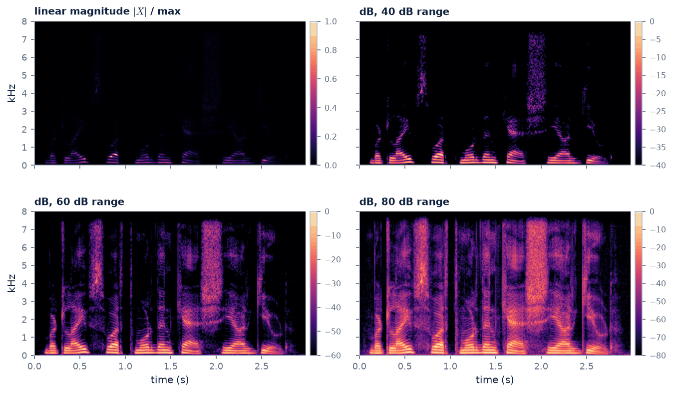
Voiced speech has strong low harmonics and formants 40–60 dB weaker higher up (see why decibels?). On a linear scale only the loudest few components show: in our sentence only 2.0 % of the time–frequency cells exceed a tenth of the peak magnitude. Taking $20\log_{10}$ compresses the range so that quiet detail becomes visible, and then we must pick a floor: everything more than $R$ dB below the maximum is drawn in the darkest colour.

The sentence drawn with a linear scale and with 40, 60 and 80 dB ranges — **Figure 7.** One spectrogram (25 ms Hann, 2 ms hop), four renderings. Linear magnitude shows little more than the low harmonics of the loudest vowels. With a 40 dB range, 14.5 % of the cells are above the floor; with 60 dB, 48.7 %; with 80 dB, 83.1 %, including the weak fricatives and the background noise in the pauses. 60–80 dB suits a clean 16-bit recording; for noisy audio a smaller range hides the noise floor.

Colour maps: why rainbows lie

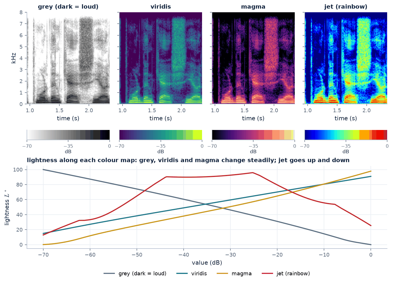
The eye judges the size of a value mostly by lightness. A good colour map changes lightness steadily from one end to the other, so equal steps in dB look like equal steps. Grey, viridis and magma are designed this way (viridis and magma are “perceptually uniform”: equal steps also look equally different in hue and saturation). The rainbow map jet is not. Its lightness climbs to a peak of $L^* \approx 96$ in the cyan-to-yellow part, about −25 dB on a 70 dB scale, then falls again to 25 at the top (dark red). So mid-level values look brighter than the loudest ones, and the sharp hue changes at cyan and yellow draw edges that are not in the data.

The same spectrogram in grey, viridis, magma and jet, and the lightness of each colour map — **Figure 8.** Part of the sentence with a 70 dB range in four colour maps, each with its colour bar. **Bottom:** lightness $L^*$ (CIELAB) along each map. Grey (dark = loud, the convention of paper spectrograms), viridis and magma change monotonically; jet rises and falls, so its bright yellow band sits in the *middle* of the range and the fricative noise looks like a solid object with a hard outline.

Whatever the map, always draw the colour bar. Without it a reader cannot tell whether dark blue means −40 dB or −80 dB, or whether the scale is linear at all, and two spectrograms with different ranges cannot be compared.

Change the scale, the range and the colour map

scale: colour map:

dynamic range (dB below the maximum that still gets a colour):

Set jet and an 80 dB range and look at the /ʃ/ of “cash, she” (about 1.8–2.1 s): it seems to have a crisp yellow border. Switch to grey or viridis: the border melts into a gradual change, which is what the numbers really do. Then drop the range to 30 dB and see which sounds vanish first.

06 · Going back to sound

Overlap-add, and the missing phase.

With the phase: exact reconstruction

The STFT keeps both magnitude and phase, and with them the signal can be rebuilt exactly. Take the inverse FFT of every column to get the windowed frames back, optionally multiply by a synthesis window $w_s$, slide each frame back to where it came from, and add. This is overlap-add (OLA), or weighted overlap-add (WOLA) when a synthesis window is used (Allen and Rabiner, 1977):

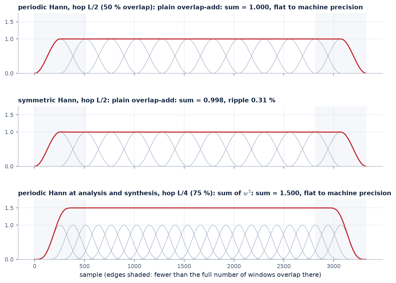
$$\hat{x}[n] = \frac{\sum_m y_m[n - mH]\; w_s[n - mH]}{\sum_m w[n - mH]\; w_s[n - mH]}, \qquad y_m[\cdot] = \text{IDFT}\bigl(X[m,\cdot]\bigr)$$ If the denominator is the same constant for every $n$, you can skip the division (or divide by that constant). For plain OLA ($w_s = 1$) the condition is COLA, “constant overlap-add”: $\sum_m w[n-mH] = C$. For WOLA with the same window twice it is $\sum_m w^2[n-mH] = C$.

Overlapping Hann windows and their sums — **Figure 9.** Shifted windows (grey) and their sum (red), $L = 512$. **Top:** a *periodic* Hann window at 50 % overlap sums to exactly 1. **Middle:** the *symmetric* Hann (as returned by `numpy.hanning`) at the same hop ripples by 0.31 %: tiny, but not exact. **Bottom:** for WOLA, Hann squared at 75 % overlap sums to exactly 1.5. (At 50 % overlap, Hann squared ripples by 66.7 %, which is why WOLA with Hann uses 75 %.)

The difference between periodic and symmetric is only the denominator, $L$ or $L-1$ in the cosine. The periodic form is one exact period of a raised cosine, and copies of it shifted by $L/2$ or $L/4$ fill each other's gaps perfectly. Tested on our sentence (47761 samples, $L = 512$):

analysis → synthesis	hop	largest sample error
periodic Hann → plain OLA	$L/2$	$5.6 \times 10^{-16}$
periodic Hann → periodic Hann (WOLA), $\div\, 1.5$	$L/4$	$4.4 \times 10^{-16}$
symmetric Hann → plain OLA	$L/2$	0.0024 (SNR 53.3 dB)

The first two errors are at the level of double-precision rounding (about $10^{-16}$ for samples of size 1): the STFT is perfectly invertible. The symmetric window's small ripple shows up as a real, if quiet, error. In practice libraries avoid the problem by dividing by the summed windows (the denominator above), which works for any window and hop as long as the windows overlap.

Without the phase: what a spectrogram cannot tell you

A spectrogram keeps only $|X|$. How much does the phase matter? Rebuild the sentence from the magnitudes ($L = 512$, $H = 128$, Hann) with made-up phases and listen:

Original

true magnitude and phase

Exact reconstruction would sound identical.

Zero phase

spectral convergence 0.87

Every frame turns into a pulse at the frame's edge, so the output repeats every hop: listen for a mechanical buzz at $f_s/H$ = 125 Hz.

Random phase

spectral convergence 0.65

The starting point of Griffin–Lim. Listen for a rough, noisy voice: overlapping frames no longer agree and partly cancel.

Griffin–Lim, 10 iterations

spectral convergence 0.218

Smoother; listen for remaining roughness.

Griffin–Lim, 100 iterations

spectral convergence 0.087

Close to the original; Griffin–Lim output typically keeps a slightly “phasey”, metallic colour.

Griffin–Lim, 200 iterations

spectral convergence 0.068

Diminishing returns: twice the work for a small gain.

All six files are scaled to the same rms level. The zero-phase output repeats every $H$ = 128 samples (its autocorrelation at that lag is 0.76), which is the buzz you hear.

Griffin–Lim: inventing the phase, one round at a time

Why can't we just pair the magnitudes with any phase? Because the frames overlap. With $H = L/4$, every sample of the signal is described by four different frames. Their phases must agree about what that sample is. Pick phases at random and the four descriptions disagree: when you add the frames back together they partly cancel, and the result's spectrogram is no longer the one you started from. A spectrogram whose frames agree is called consistent: it is the STFT of some real signal. Most arrays of numbers are not.

So the puzzle has two requirements, and each one on its own is easy to meet:

$\mathcal{A}$: the right magnitudes

All arrays $S[m,k]\,e^{j\phi[m,k]}$: keep the target magnitudes $S$, any phase. Easy to reach from any array: replace its magnitudes by $S$, keep its phase.

$\mathcal{B}$: consistent spectrograms

All arrays that are the STFT of a real signal. Easy to reach from any array: inverse-STFT it, then STFT the result.

We want an array that lies in both. Griffin and Lim's idea (1984) is to bounce between the two sets: step onto $\mathcal{B}$, step back onto $\mathcal{A}$, and repeat. Each step moves to the nearest point of the other set, so the distance between where you are and where you were can only shrink:

Figure 10. Alternating projections, drawn schematically. Each red arrow moves to the nearest point of the other set. Steps get shorter as the two descriptions agree more. The real sets live in a space with one dimension per time–frequency cell (here about 96375 of them), and they are not straight lines, so the zigzag can settle near, rather than exactly at, a crossing.

The algorithm, step by step

Given: the target magnitudes $S[m,k]$, the window $w$ (length $L$) and the hop $H$ used to make them. Wanted: a signal $y[n]$ with $|\text{STFT}(y)| \approx S$.

Guess a phase. Start from random phases, uniform on $[-\pi, \pi)$: $$\phi^{(0)}[m,k] \sim \mathcal{U}[-\pi, \pi)$$
Attach it to the magnitudes (we are on $\mathcal{A}$): $$X^{(i)}[m,k] = S[m,k]\; e^{\,j\phi^{(i)}[m,k]}$$
Go back to a waveform by overlap-add. Griffin and Lim showed that, of all signals, this one has the STFT closest (in squared error) to $X^{(i)}$: $$y^{(i)}[n] = \frac{\sum_m w[n - mH]\; \text{IDFT}\bigl(X^{(i)}[m,\cdot]\bigr)[n - mH]}{\sum_m w^2[n - mH]}$$
Analyse it again (we are now on $\mathcal{B}$: consistent, but the magnitudes have drifted away from $S$): $$Z^{(i)}[m,k] = \text{STFT}\bigl(y^{(i)}\bigr)[m,k]$$
Keep the new phase, throw away the new magnitude, and go back to step 2: $$\phi^{(i+1)}[m,k] = \angle\, Z^{(i)}[m,k]$$

Track progress with the spectral convergence $\;\mathrm{SC}^{(i)} = \bigl\|\,S - |Z^{(i)}|\,\bigr\|_F \,/\, \|S\|_F$, where $\|\cdot\|_F$ is the square root of the sum of squares over all cells. Stop when it stops falling; the answer is $y^{(i)}$.

# Griffin-Lim in a few lines (numpy + librosa-style stft/istft)
phase = np.exp(2j * np.pi * np.random.rand(*S.shape))      # step 1
for i in range(n_iter):
    y = istft(S * phase, hop=H, window=w)                    # steps 2-3
    Z = stft(y, hop=H, window=w)                             # step 4
    phase = np.exp(1j * np.angle(Z))                         # step 5

Why it can never get worse. Let $d^{(i)} = \|Z^{(i)} - X^{(i)}\|_F$ be the gap between the consistent array and the one with the right magnitudes. Step 5 picks the point of $\mathcal{A}$ nearest to $Z^{(i)}$ (same phase, magnitudes reset to $S$), and step 3 picks the point of $\mathcal{B}$ nearest to that. A nearest point can only be closer than any other point, including the one you came from, so $d^{(i+1)} \le d^{(i)}$ at every round. Griffin and Lim proved exactly this. What they could not promise is that the gap reaches zero: it can stall at a local minimum.

Think of each sample as a meeting of the four frames that overlap it. With random phases, each frame argues for a different value and the votes cancel into mush. Overlap-add takes the average, which is a compromise. When each frame then re-reads the phase from that compromise, it moves a little towards agreeing with its neighbours. Small agreements spread from frame to frame, a bit like a crowd's clapping falling into step. After a few dozen rounds the harmonics line up across frames and the voice comes back.

Live: watch Griffin–Lim learn the phase

The page takes the magnitudes of our sentence ($L = 512$, $H = 128$, periodic Hann), throws the phase away and runs the five steps above in your browser. The spectrogram on the left is $|Z^{(i)}|$, what the current estimate really contains; the target is on the right. Press Run and listen at any point.

start from: fast Griffin–Lim (momentum 0.99)

current estimate $|Z^{(i)}|$

target $S$ (the magnitudes we kept)

spectral convergence vs iteration (log scale)

30 ms of the vowel in “cash”: original (grey) and current estimate

Things to notice: the first few rounds give the biggest jump; the harmonics in the vowels come back as clean horizontal lines over the first few tens of rounds; and the waveform never matches the original sample for sample, even when the spectrogram does, because many waveforms share one spectrogram (the sign of the whole signal, for a start). With momentum ticked (Perraudin, Balazs and Søndergaard, 2013) each round also pushes a little further in the direction the last round moved: in our offline run it matched 100 plain rounds after only 21 rounds, and reached a spectral convergence of 0.019 after 200 (plain: 0.068).

The numbers from a longer run

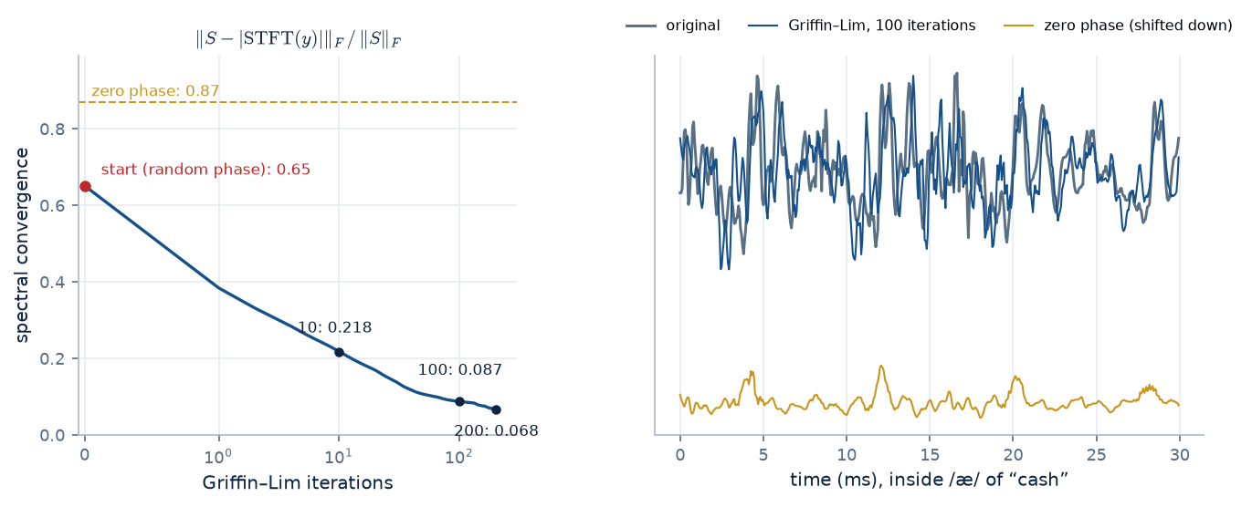
Griffin-Lim spectral convergence against iterations, and waveforms — **Figure 11.** **Left:** spectral convergence falls from 0.65 (random phase) to 0.38 after one iteration, 0.218 after 10, 0.087 after 100 and 0.068 after 200. It fell at every single iteration of our run. With the true phase it is $2.2 \times 10^{-16}$. **Right:** 30 ms of the vowel in “cash”. The Griffin–Lim waveform (100 iterations) has nearly the same spectrogram as the original but a visibly different waveform: many waveforms share one magnitude.

Griffin–Lim never quite reaches zero: it is a local search, not every magnitude array is the STFT of any signal, and some differences (an overall sign flip, for one) are invisible in $|X|$. For decades it was the standard way to hear a modified spectrogram. Today, text-to-speech systems first predict a mel spectrogram (section 8) and then use a neural vocoder (WaveNet, WaveRNN, HiFi-GAN and their successors), a network trained to generate a natural-sounding waveform, phase included, from it.

07 · Reading speech

Phones you can see.

With a wideband spectrogram, and a little practice, you can see the classes of speech sounds. Each class has a typical look because each is made in a typical way (the source–filter model): a voiced buzz or a turbulent hiss as the source, shaped by the resonances of the vocal tract.

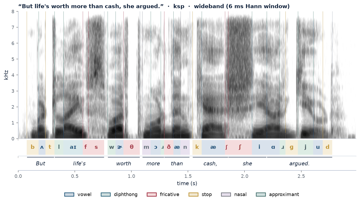
Wideband spectrogram of the sentence with IPA phone labels and words — **Figure 12.** The sentence in a 6 ms wideband view (grey, dark = loud, 70 dB range) with the corpus's phone labels in IPA, coloured by class. The labels were made automatically by a speech aligner and were not hand-corrected, so some boundaries are off by a frame or two (we merged one 10 ms pause the aligner put inside “cash, she”).

Hover to read, click to listen

click plays:

phonehover or tap the spectrogram

A single phone played alone often sounds odd or is hard to recognise: in fluent speech each sound is shaped by its neighbours (coarticulation). Try the word as well.

A gallery of sound classes

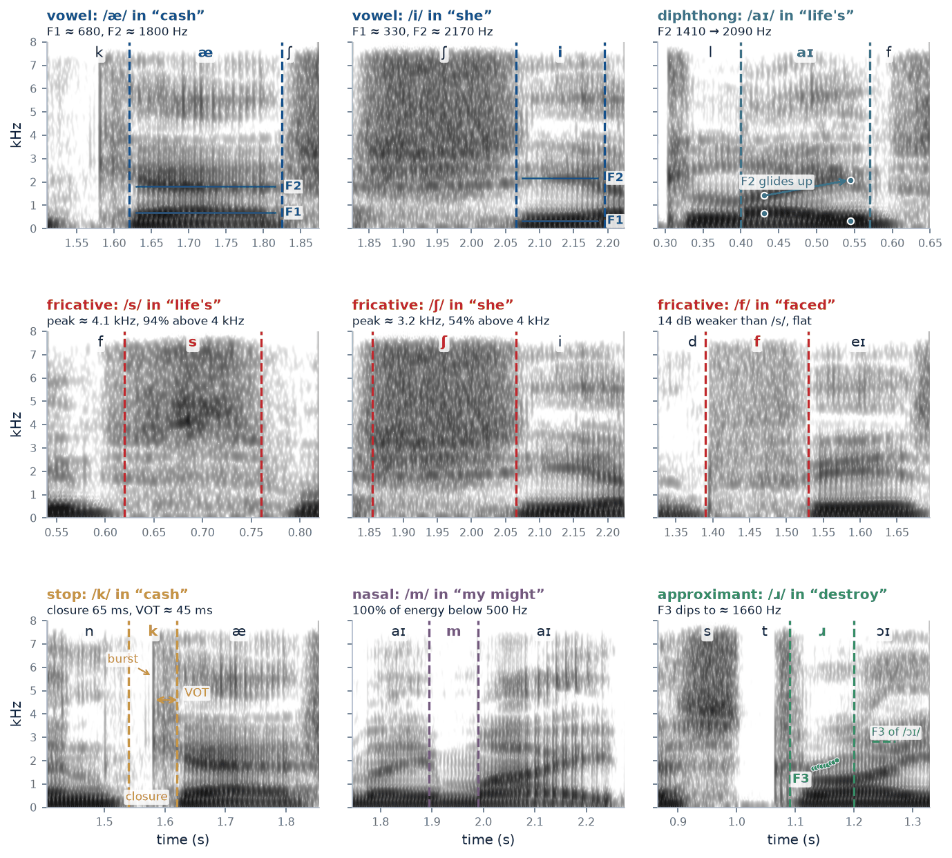
Nine wideband spectrogram excerpts: vowels, a diphthong, three fricatives, a stop, a nasal and an approximant — **Figure 13.** Nine tokens of ksp's speech, each with its neighbours, in the same 6 ms wideband view and on *one common dB scale* (so weak sounds look weak). Dashed lines mark the labelled boundaries. The numbers above each panel were measured from the audio by `make_figures.py` (formants by linear prediction), as a check on the automatic labels. Seven tokens come from our sentence; /f/ is from “faced”, /m/ from “all my might” and /ɹ/ from “destroy”.

vowel /æ/ “cash”

vowel /i/ “she”

diphthong /aɪ/ “life's”

fricative /s/ “life's”

fricative /ʃ/ “she”

fricative /f/ “faced”

stop /k/ “cash”

nasal /m/ “my might”

approximant /ɹ/ “destroy”

Vowels: dark bands and striations

Vowels are voiced and the tract is open, so a wideband view shows vertical glottal striations under dark horizontal formant bands, the resonances $F_1, F_2, F_3$. $F_1$ goes up as the jaw opens; $F_2$ goes up as the tongue moves forward. Open front /æ/ in “cash” has $F_1 \approx 680$ Hz and $F_2 \approx 1800$ Hz; close front /i/ in “she” has a low $F_1$ ($\approx 330$ Hz) and a high $F_2$ ($\approx 2170$ Hz). In a narrowband view the same vowels are stacks of harmonics, and the formants are the regions where the harmonics are strongest.

Diphthongs: formants on the move

A diphthong glides from one vowel to another, so its formants move. In /aɪ/ of “life's” $F_1$ falls from about 650 to 340 Hz and $F_2$ rises from about 1410 to 2090 Hz, from an open /a/ towards a close front /ɪ/.

Fricatives: noise, and where it sits

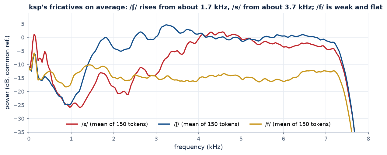
Fricatives are turbulent noise from a narrow constriction, so they look like random speckle with no striations (unless voiced, like /z/ or /v/). The smaller the cavity in front of the constriction, the higher the noise. In ksp's /s/ of “life's” 94 % of the energy above 500 Hz lies above 4 kHz (spectral peak near 4090 Hz). /ʃ/, with lip rounding and a longer front cavity, starts lower: its peak in “she” is near 3220 Hz and only 54 % of its energy is above 4 kHz. /f/ and /θ/ have almost no front cavity: their noise is weak and spread flat; ksp's /f/ in “faced” is 13.7 dB weaker than the /s/.

Average spectra of ksp's s, sh and f — **Figure 14.** The same contrast averaged over the 150 longest tokens of each fricative in ksp's recordings (20 ms Hann frames from the middle of each token). /ʃ/ comes within 6 dB of its maximum from about 1700 Hz, /s/ only from about 3700 Hz; /f/ stays flat and on average 10 dB weaker than /s/. (This speaker's /s/ is broad, reaching up to the 7.5 kHz limit of the recording; in many English speakers it peaks higher still.)

Stops: silence, a click, then the vowel

A stop is a complete closure, so it shows as a gap: near silence (a faint voice bar at the bottom if the stop is voiced). The release is a burst, a thin vertical line across many frequencies. Then comes the time until the vocal folds start vibrating, the voice onset time (VOT), filled with aspiration noise for aspirated stops. For /k/ in “cash” the closure lasts about 65 ms (22 dB weaker than the following vowel), the burst comes at 1.58 s and voicing starts about 45 ms later; across 97 of ksp's /k/ tokens before a vowel the median VOT is 51 ms. Compare /b/ in “But”, where voicing follows the burst after about 3 ms. The place of articulation shows in the burst's spectrum and in how the formants bend into the next vowel.

Nasals: a low murmur with the top cut off

In a nasal the mouth is closed and sound leaves through the nose. The long nasal tract gives a strong resonance low down (the nasal murmur), and the closed mouth acts as a side branch that traps energy at some frequencies (antiresonances, zeros of the transfer function), so the upper formants are weak. In /m/ of “my might” 100 % of the energy lies below 500 Hz (the following vowel /aɪ/: 23 %), and the 1–3 kHz region is 33 dB weaker than in the vowel. The edges are abrupt, because the lips close and open quickly.

Approximants: vowel-like, but moving

/w, j, ɹ, l/ are made with a narrowing that is too wide for noise, so they look like weak vowels whose formants move into the next sound. /w/ has a low $F_2$, /j/ a high $F_2$, and the English /ɹ/ is famous for a very low $F_3$. In “destroy” ksp's $F_3$ dips to about 1660 Hz, against about 2820 Hz in the following /ɔɪ/. That dip is weaker in many Indian-English accents, where /r/ is often a tap or a lighter approximant rather than the bunched or retroflex /ɹ/ of American English: across the 300 longest /r/ tokens of ksp the median lowest $F_3$ is about 2430 Hz, and only 22 % go below 2.2 kHz. Spectrograms show accents too.

Read a speech spectrogram in three passes. Where is the energy in time? Gaps are stop closures or pauses; vertical lines are bursts. Is it periodic or noisy? Striations (or harmonics) mean voicing; speckle means friction. Where is it in frequency? Formant positions name the vowel; the lower edge of the noise names the fricative; a strong low band with a weak top suggests a nasal.

purpose	sample rate	window	hop	FFT size	then
reading phonetics (wideband)	16 kHz	3–6 ms Hann	1 ms	256–512	dB, 60–80 dB range, grey
pitch and harmonics (narrowband)	16 kHz	30–50 ms Hann	5–10 ms	1024–2048	dB, often 0–4 kHz only
speech recognition features	16 kHz	25 ms (400 samples) Hamming or Hann	10 ms (160)	400–512	80–128 mel bands, log (Kaldi-style filterbanks; Whisper uses 80, its large-v3 model 128)
neural TTS vocoder input	22.05–24 kHz	\(\approx 46\) ms (1024 samples) Hann	\(\approx 11.6\) ms (256)	1024	80 mel bands, log (e.g. HiFi-GAN)
telephone speech	8 kHz	20–32 ms Hamming	10 ms	256	only 0–4 kHz exists
music analysis	44.1–48 kHz	\(\approx 46\) ms (2048) Hann	\(\approx 11.6\) ms (512)	2048–4096	dB or log-frequency (constant-Q)

09 · Check your understanding

Six questions.

1. At 16 kHz you use 20 ms frames and a 512-point FFT. What is the bin spacing, and can you separate two tones 40 Hz apart? What would you change?

Bin spacing $16000/512 = 31.25$ Hz. But the resolution is set by $L = 320$ samples: $f_s/L = 50$ Hz per bin of the window, and a Hann window needs about 2 such bins (100 Hz) to separate two equal tones. So no. A bigger FFT will not help (Figure 3); a longer window will: about $2 \times 16000/40 = 800$ samples, 50 ms.

2. A child speaks with $F_0 = 300$ Hz. What window lengths give a wideband and a narrowband view? Is the usual 25 ms window wideband or narrowband for this child?

$T_0 = 1/300 \approx 3.3$ ms. Wideband needs $L < T_0$, say 2 ms (32 samples at 16 kHz). Narrowband needs two or three periods or more, from about 7–10 ms. A 25 ms window covers 7.5 periods: strongly narrowband. For high voices, “standard” settings resolve harmonics, not formants, which is one reason formant tracking is harder for children's speech.

3. A spectrogram of a whistle drawn with a rectangular window shows a bright line with a faint haze above and below it across the whole picture. Where does the haze come from?

Leakage. The rectangular window's spectrum has side lobes starting at about −13.3 dB that fall only 6 dB per octave, so the strong line spreads into every bin. A Hann window's side lobes start at −31.5 dB and fall 18 dB per octave, so the haze disappears into the floor.

4. On a spectrogram drawn with a 40 dB range you cannot find the /f/ of “faced”. Was the /f/ missing?

Probably not. /f/ is weak: about 14 dB below this speaker's /s/, and the /s/ is itself far below the loudest vowel bins. With only 40 dB between the brightest and darkest colours the /f/ falls under the floor. Increase the range to 60–80 dB (Figure 7, and the colour demo).

5. You analyse with numpy's hanning(512), hop 256, and resynthesise by plain overlap-add. The result is close but not exact. Why, and give two fixes.

numpy.hanning is the symmetric Hann window, whose shifted copies at 50 % overlap sum to a constant only approximately (ripple 0.31 %, error SNR 53.3 dB on our sentence). Fix 1: use the periodic Hann (scipy.signal.get_window('hann', 512)), which is COLA at hop $L/2$. Fix 2: divide the overlap-added output by the summed windows, which makes any window work.

6. After 100 iterations Griffin–Lim reaches a spectral convergence of 0.087, not 0. Give two reasons why it cannot simply recover the original waveform.

(a) Different signals share the same STFT magnitude: at the very least $x$ and $-x$, so the original is not the only answer. (b) Griffin–Lim is a local, alternating search started from random phase: each step cannot make things worse, but it can settle in a poor, “phasey” solution that is not globally best. (Also, once a spectrogram has been edited or predicted by a model, it may not be the magnitude of any signal, and then no phase gives zero error.)

symbol	name	what it controls	typical for speech at 16 kHz
\(L\)	window length	how long a slice the analysis “sees”, and so the trade-off between time detail and frequency detail (section 4)	5–40 ms (80–640 samples)
\(H\)	hop	how often a column is computed; it sets the picture's time sampling but not its time resolution	1–10 ms, usually \(L/4\) to \(L/2\)
\(N\)	FFT size	how many frequency points are drawn: the bin spacing is \(f_s/N\)	the next power of two \(\ge L\), e.g. 512

analysis → synthesis	hop	largest sample error
periodic Hann → plain OLA	\(L/2\)	\(5.6 \times 10^{-16}\)
periodic Hann → periodic Hann (WOLA), \(\div\, 1.5\)	\(L/4\)	\(4.4 \times 10^{-16}\)
symmetric Hann → plain OLA	\(L/2\)	0.0024 (SNR 53.3 dB)